Exploring the Effects of Dimensionality on a PDF of Distances
Every so often I’m reminded that the effects of changing dimensionality on objects and processes can be surprisingly counterintuitive. Recently I ran across a great example of this, while I working on a model for the distribution of distances in spaces of varying dimension.
Suppose that I draw some values from a classic one-dimensional Gaussian, with zero mean and unit variance, but that I am actually interested in their corresponding distances from center. Knowing that my Gaussian is centered on the origin, I can rephrase that as: the distribution of magnitudes of values drawn from that Gaussian. I can simulate this process by actually samping Gaussian values and taking their absolute value. When I do, I get the following result:
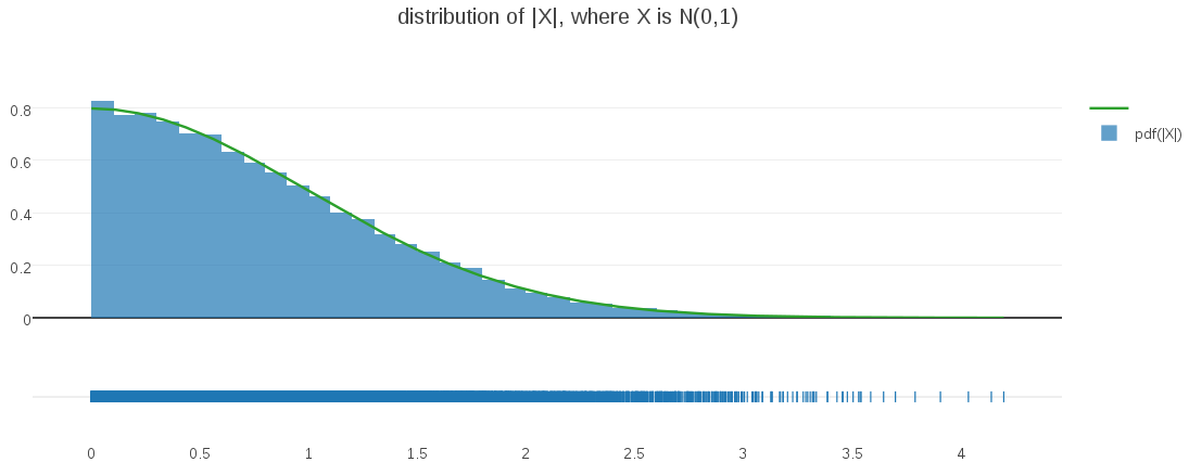
It’s easy to see – and intuitive – that the resulting distribution is a half-Gaussian, as I confirmed by overlaying the histogrammed samples above with a half-Gaussian PDF (displayed in green).
I wanted to generalize this basic idea into some arbitrary dimensionality, (d), where I draw d-vectors from an d-dimensional Gaussian (again, centered on the origin with unit variances). When I take the magnitudes of these sampled d-vectors, what will the probability distribution of their magnitudes look like?
My intuitive assumption was that these magnitudes would also follow a half-Gaussian distribution. After all, every multivariate Gaussian is densest at its mean, just like the univariate case I examined above. In fact I was so confident in this assumption that I built my initial modeling around it. Great confusion ensued, when I saw how poorly my models were working on my higher-dimensional data!
Eventually it occurred to me to do the obvious thing and generate some visualizations from higher dimensional data. For example, here is the correponding plot generated from a bivariate Gaussian (d=2):
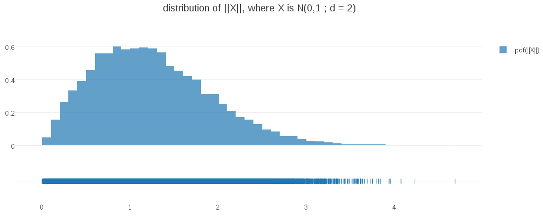
Surprise – the distribution at d=2 is not even close to half-Gaussian!. My intuitions couldn’t have been more misleading!
Where did I go wrong?
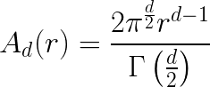
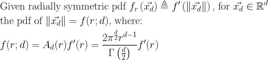
I’ll start by observing what happens when I take a multi-dimensional PDF of vectors in (d) dimensions and project it down to a one-dimensional PDF of the corresponding vector magnitudes. To keep things simple, I will be assuming a multi-dimensional PDF \(f_r(\vec{x_d})\) that is (1) centered on the origin, and (2) is radially symmetric; the pdf value is the same for all points at a given distance from the origin. For example, any multivariate Gaussian with \(\vec{0_d}\) mean and \(I_d\) for a covariance matrix satisfies these two assumptions. With this in mind, you can see that the process of projecting from vectors in \(R_d\) to their distance from \(\vec{0_d}\) (their magnitude) is equivalent to summing all densities \(f_r(\vec{x_d})\) along the surface of “d-sphere” radius (r) to obtain a pdf \(f(r)\) in distance space. With assumption (2) we can simplify that integration to just \(f(r) = A_d(r)f'(r)\) , where \(f'(r)\) defines the value of \(f_r(\vec{x})\) for all \(\vec{x}\) with magnitude of (r), and \(A_d(r)\) is the surface area of a d-sphere with radius (r):
The key observation is that this term is a polynomial function of radius (r), with degree (d-1). When d=1, it is simply a constant multiplier and so we get the half-Gaussian distribution we expect, but when
The above ideas can be expressed compactly as follows:
In my experiments, I am using multivariate Gaussians of mean \(\vec{0_d}\) and unit covariance matrix \(I_d\) , and so the form for \(f(r;d)\) becomes:
This form is in fact the generalized gamma distribution, with scale parameter \(a = \sqrt{2}\) , shape parameter \(p = 2\), and free shape parameter (d) representing the dimensionality in this context.
I can verify that this PDF is correct by plotting it against randomly sampled data at differing dimensions:
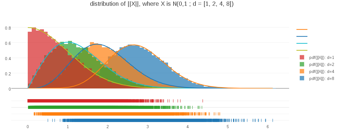
This plot demonstrates both that the PDF expression is correct for varying dimensionalities and also illustrates how the shape of the PDF evolves as dimensionality changes. For me, it was a great example of challenging my intuitions and learning something completely unexpected about the interplay of distances and dimension.