Implementing Parallel Prefix Scan as a Spark RDD Transform
In my previous post, I described how to implement the Scala scanLeft function as an RDD transform. By definition scanLeft invokes a sequential-only prefix scan algorithm; it does not assume that either its input function f or its initial-value z can be applied in a parallel fashion. Its companion function scan, however, computes a parallel prefix scan. In this post I will describe an implementation of parallel prefix scan as an RDD transform.
As was the case with scanLeft, a basic strategy is to begin by applying scan to each RDD partition. Provided that appropriate “offsets” {z1, z2, ...} can be computed for each partition, these can be applied to the partial, per-partition results to yield the output. In fact, the desired {z1, z2, ...} are the parallel prefix scan of the last element in each per-partition scan. The following diagram illustrates:
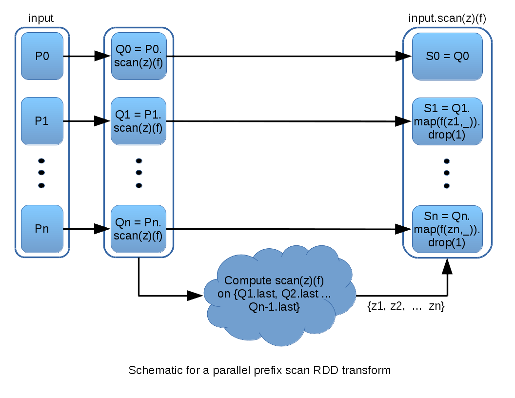
The diagram above glosses over the details of computing scan to obtain {z1, z2, ...}. I will first describe the implementation I currently use, and then also discuss a possible alternative. The current implementation takes the approach of encoding the logic of a parallel prefix scan directly into an RDD computation DAG. Each iteration, or “ply,” of the parallel algorithm is represented by an RDD. Each element resides in its own partition, and so the computation dependency for each element is directly representable in the RDD dependency substructure. This construction is illustrated in the following schematic (for a vector of 8 z-values):
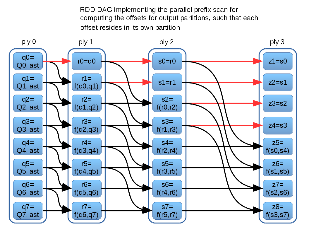
The parallel prefix scan algorithm executes O(log(n)) plies, which materializes as O(log(n)) RDDs shown in the diagram above. In this context, (n) is the number of input RDD partitions, not to be confused with the number of data rows in the RDD. There are O((n)log(n)) partitions, each having a single row containing the z-value for a corresponding output partition. Some z-values are determined earlier than others. For example z1 is immediately available in ply(0), and ply(3) can refer directly back to that ply(0) partition in the interest of efficiency, as called out by the red DAG arcs.
This scheme allows each final output partition to obtain its z-value directly from a single dedicated partition, which ensures that minimal data needs to be transferred across worker processes. Final output partitions can be computed local to their corresponding input partitions. Data transfer may be limited to the intermediate z-values, which are small single-row affairs by construction.
The code implementing the logic above can be viewed here.
I will conclude by noting that there is an alternative to this highly distributed computation of {z1, z2, ...}, which is to collect the last-values in the per-partition intermediate scan ouputs into a single array, and run scan directly on that array. This has the advantage of avoiding the construction of log(n) intermediate RDDs. It does, however, require a monolithic ‘fan-in’ of data into a single RDD to receive the collection of values. That is followed by a fan-out of the array, where each output partition picks its single z-value from the array. It is for this reason I suspect this alternative incurs substantially more transfer overhead across worker processes. However, one might also partition the resulting z-values in some optimal way, so that each final output partition needs to request only the partition that contains its z-value. Future experimentation might show that this can out-perform the current fully-distributed implementation.