Solving Feasible Points With Smooth-Max
Overture
Lately I have been fooling around with an implementation of the Barrier Method for convex optimization with constraints. One of the characteristics of the Barrier Method is that it requires an initial-guess from inside the feasible region: that is, a point which is known to satisfy all of the inequality constraints provided by the user. For some optimization problems, it is straightforward to find such a point by using knowledge about the problem domain, but in many situations it is not at all obvious how to identify such a point, or even if a feasible point exists. The feasible region might be empty!
Boyd and Vandenberghe discuss a couple approaches to finding feasible points in §11.4 of [1].
These methods require you to set up an “augmented” minimization problem:
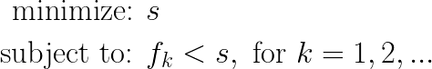
As you can see from the above, you have to set up an “augmented” space x+s, where (s) represents an additional dimension, and constraint functions are augmented to fk-s
The Problem
I experimented a little with these, and while I am confident they work for most problems having multiple inequality constraints, my unit testing tripped over an ironic deficiency: when I attempted to solve a feasible point for a single planar constraint, the numerics went a bit haywire. Specifically, a linear constraint function happens to have a singular Hessian of all zeroes. The final Hessian, coming out of the log barrier function, could be consumed by SVD to get a search direction but the resulting gradients behaved poorly.
Part of the problem seems to be that the nature of this augmented minimization problem forces the algorithms to push (s) ever downward, but letting (s) transitively push the fk with the augmented constraint functions fk-s. When only a single linear constraint function is in play, the resulting gradient caused augmented dimension (s) to converge against the movement of the remaining (unaugmented) sub-space. The minimization did not converge to a feasible point, even though literally half of the space on one side of the planar surface is feasible!
Smooth Max
Thinking about these issues made me wonder if a more direct approach was possible. Another way to think about this problem is to minimize the maximum fk; If the maximum fk is < 0 at a point x, then x is a feasible point satisfying all fk. If the smallest-possible maximum fk is > 0, then we have definitive proof that no feasible point exists, and our constraints can’t be satisfied.
Taking a maximum preserves convexity, which is a good start, but maximum isn’t differentiable everywhere. The boundaries between regions where different functions are the maximum are not smooth, and along those boundaries there is no gradient, and therefore no Hessian either.
However, there is a variation on this idea, known as smooth-max, defined like so:
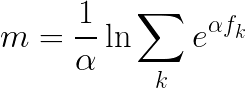
Smooth-max has a well defined gradient and Hessian, and furthermore can be computed in a numerically stable way. The sum inside the logarithm above is a sum of exponentials of convex functions. This is good news; exponentials of convex functions are log-convex, and a sum of log-convex functions is also log-convex.
That means I have the necessary tools to set up the my mini-max problem: For a given set of convex constraint functions fk, I create a functions which is the soft-max of these, and I minimize it.
Go Directly to Jail
I set about implementing my smooth-max idea, and immediately ran into almost the same problem as before. If I try to solve for a single planar constraint, my Hessian degenerates to all-zeros! When I unpacked the smoothmax-formula for a single constraint fk, it indeed is just fk, zero Hessian and all!
More is More
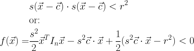
What to do? Well you know what form of constraint always has a well behaved Hessian? A circle, that’s what. More technically, an n-dimensional ball, or n-ball. What if I add a new constraint of the form:
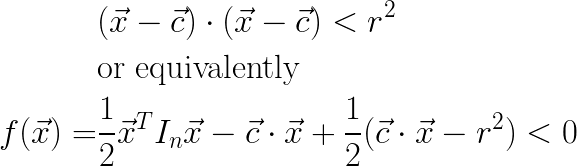
This constraint equation is quadratic, and its Hessian is In. If I include this in my set of constraints, my smooth-max Hessian will be non-singular!
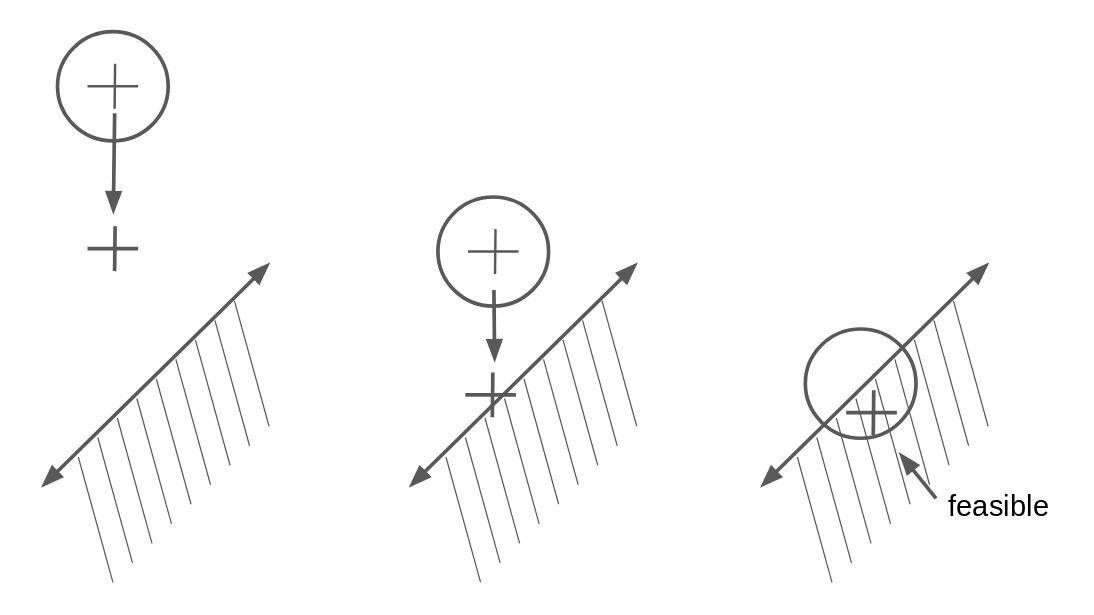
Since I do not know a priori where my feasible point might lie, I start with my n-ball centered at my initial guess, and minimize. The result might look something like this:
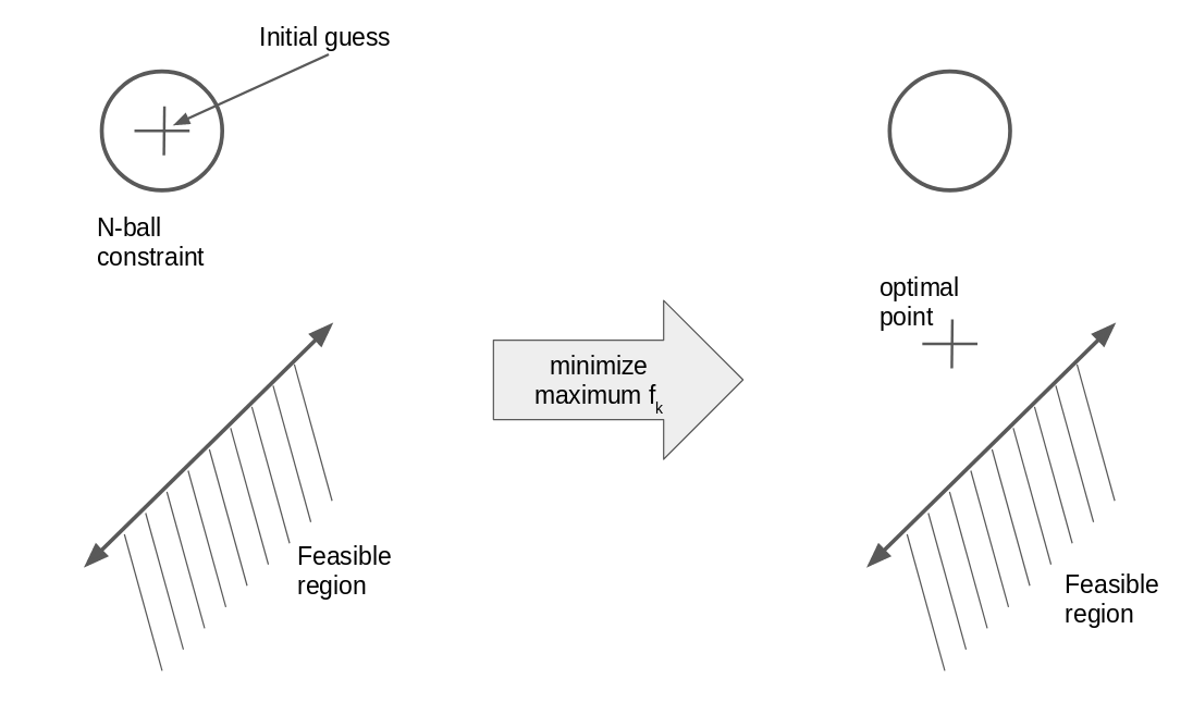
Because the optimization is minimizing the maximum fk, the optimal point may not be feasible, but if not it will end up closer to the feasible region than before. This suggests an iterative algorithm, where I update the location of the n-ball at each iteration, until the resulting optimized point lies on the intersection of my original constraints and my additional n-ball constraint:
Caught in the Underflow
I implemented the iterative algorithm above (you can see what this loop looks like here), and it worked exactly as I hoped… at least on my initial tests. However, eventually I started playing with its convergence behavior by moving my constraint region farther from the initial guess, to see how it would cope. Suddenly the algorithm began failing again. When I drilled down on why, I was taken aback to discover that my Hessian matrix was once again showing up as all zeros!
The reason was interesting. Recall that I used a modified formula to stabilize my smooth-max computations. In particular, the “stabilized” formula for the Hessian looks like this:
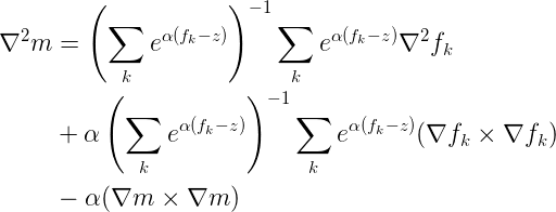
So, what was going on? As I started moving my feasible region farther away, the corresponding constraint function started to dominate the exponential terms in the equation above. In other words, the distance to the feasible region became the (z) in these equations, and this z value was large enough to drive the terms corresponding to my n-ball constraint to zero!
However, I have a lever to mitigate this problem. If I make the α parameter small enough, it will compress these exponent ranges and prevent my n-ball Hessian terms from washing out. Decreasing α makes smooth-max more rounded-out, and decreases the sharpness of the approximation to the true max, but minimizing smooth-max still yields the same minimum location as true maximum, and so playing this trick does not undermine my results.
How small is small enough? α is essentially a free parameter, but I found that if I set it at each iteration, such that I make sure that my n-ball Hessian coefficient never drops below 1e-3 (but may be larger), then my Hessian is always well behaved. Note that as my iterations grow closer to the true feasible region, I can gradually allow α to grow larger. Currently, I don’t increase α larger than 1, to avoid creating curvatures too large, but I have not experimented deeply with what actually happens if it were allowed to grow larger. You can see what this looks like in my current implementation here.
Convergence
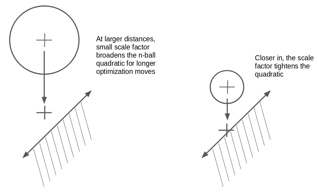
Tuning the smooth-max α parameter gave me numeric stability, but I noticed that as the feasible region grew more distant from my initial guess, the algorithm’s time to converge grew larger fairly quickly. When I studied its behavior, I saw that at large distances, the quadratic “cost” of my n-ball constraint effectively pulled the optimal point fairly close to my n-ball center. This doesn’t prevent the algorithm from finding a solution, but it does prevent it from going long distances very fast. To solve this adaptively, I added a scaling factor s to my n-ball constraint function. The scaled version of the function looks like:
In my case, when my distances to a feasible region grow large, I want s to become small, so that it causes the cost of the n-ball constraint to grow more slowly, and allow the optimization to move farther, faster. The following diagram illustrates this intuition:
In my algorithm, I set s = 1/σ, where σ represents the “scale” of the current distance to feasible region. The n-ball function grows as the square of the distance to the ball center; therefore I set σ=(k)sqrt(s), so that it grows proportionally to the square root of the current largest user constraint cost. Here, (k) is a proportionality constant. It too is a somewhat magic free parameter, but I have found that k=1.5 yields fast convergences and good results. One last trick I play is that I prevent σ from becoming less than a minimum value, currently 10. This ensures that my n-ball constraint never dominates the total constraint sum, even as the optimization converges close to the feasible region. I want my “true” user constraints to dominate the behavior near the optimum, since those are the constraints that matter. The code is shorter than the explaination: you can see it here
Conclusion
After applying all these intuitions, the resulting algorithm appears to be numerically stable and also converges pretty quickly even when the initial guess is very far from the true feasible region. To review, you can look at the main loop of this algorithm starting here.
I’ve learned a lot about convex optimization and feasible point solving from working through practical problems as I made mistakes and fixed them. I’m fairly new to the whole arena of convex optimization, and I expect I’ll learn a lot more as I go. Happy Computing!
References
[1] §11.3 of Convex Optimization, Boyd and Vandenberghe, Cambridge University Press, 2008