Using Minimum Description Length to Optimize the 'K' in K-Medoids
Applying many popular clustering models, for example K-Means, K-Medoids and Gaussian Mixtures, requires an up-front choice of the number of clusters – the ‘K’ in K-Means, as it were. Anybody who has ever applied these models is familiar with the inconvenient task of guessing what an appropriate value for K might actually be. As the size and dimensionality of data grows, estimating a good value for K rapidly becomes an exercise in wild guessing and multiple iterations through the free-parameter space of possible K values.
There are some varied approaches in the community for addressing the task of identifying a good number of clusters in a data set. In this post I want to focus on an approach that I think deserves more attention than it gets: Minimum Description Length.
Many years ago I ran across a superb paper by Stephen J. Roberts on anomaly detection that described a method for automatically choosing a good value for the number of clusters based on the principle of Minimum Description Length. Minimum Description Length (MDL) is an elegant framework for evaluating the parsimony of a model. The Description Length of a model is defined as the amount of information needed to encode that model, plus the encoding-length of some data, given that model. Therefore, in an MDL framework, a good model is one that allows an efficient (i.e. short) encoding of the data, but whose own description is also efficient (This suggests connections between MDL and the idea of learning as a form of data compression).
For example, a model that directly memorizes all the data may allow for a very short description of the data, but the model itself will cleary require at least the size of the raw data to encode, and so direct memorization models generaly stack up poorly with respect to MDL. On the other hand, consider a model of some Gaussian data. We can describe these data in a length proportional to their log-likelihood under the Gaussian density. Furthermore, the description length of the Gaussian model itself is very short; just the encoding of its mean and standard deviation. And so in this case a Gaussian distribution represents an efficient model with respect to MDL.
In summary, an MDL framework allows us to mathematically capture the idea that we only wish to consider increasing the complexity of our models if that buys us a corresponding increase in descriptive power on our data.
In the case of Roberts’ paper, the clustering model in question is a Gaussian Mixture Model (GMM), and the description length expression to be optimized can be written as:
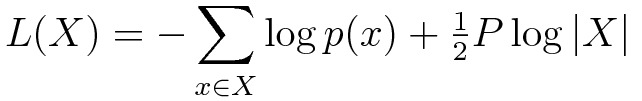
In this expression, X represents the vector of data elements.
The first term is the (negative) log-likelihood of the data, with respect to a candidate GMM having some number (K) of Gaussians; p(x) is the GMM density at point (x).
This term represents the cost of encoding the data, given that GMM.
The second term is the cost of encoding the GMM itself.
The value P is the number of free parameters needed to describe that GMM.
Assuming a dimensionality D for the data, then
I wanted to apply this same MDL principle to identifying a good value for K, in the case of a K-Medoids model. How best to adapt MDL to K-Medoids poses some problems. In the case of K-Medoids, the only structure given to the data is a distance metric. There is no vector algebra defined on data elements, much less any ability to model the points as a Gaussian Mixture.
However, any candidate clustering of my data does give me a corresponding distribution of distances from each data element to it’s closest medoid. I can evaluate an MDL measure on these distance values. If adding more clusters (i.e. increasing K) does not sufficiently tighten this distribution, then its description length will start to increase at larger values of K, thus indicating that more clusters are not improving our model of the data. Expressing this idea as an MDL formulation produces the following description length formula:
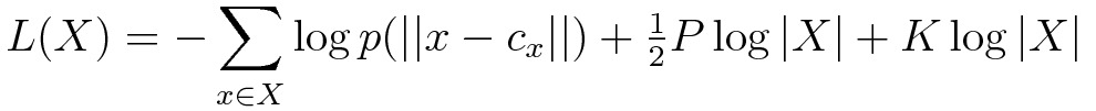
Note that the first two terms are similar to the equation above; however, the underlying distribution
And so, an MDL-based algorithm for automatically identifying a good number of clusters (K) in a K-Medoids model is to run a K-Medoids clustering on my data, for some set of potential K values, and evaluate the MDL measure above for each, and choose the model whose description length L(X) is the smallest!
As I mentioned above, there is also an implied task of choosing a form (or a set of forms) for the distance distribution
Another observation (based on my blog posts mentioned above) is that my use of the gamma distribution implies a bias toward cluster distributions that behave (more or less) like Gaussian clusters, and so in this respect its current behavior is probably somewhat analogous to the G-Means algorithm, which identifies clusterings that yield Gaussian disributions in each cluster. Adding other candidates for distance distributions is a useful subject for future work, since there is no compelling reason to either favor or assume Gaussian-like cluster distributions over all kinds of metric spaces. That said, I am seeing reasonable results even on data with clusters that I suspect are not well modeled as Gaussian distributions. Perhaps the shape-coverage of the gamma distribution is helping to add some robustness.
To demonstrate the MDL-enhanced K-Medoids in action, I will illustrate its performance on some data sets that are amenable to graphic representation. The code I used to generate these results is here.
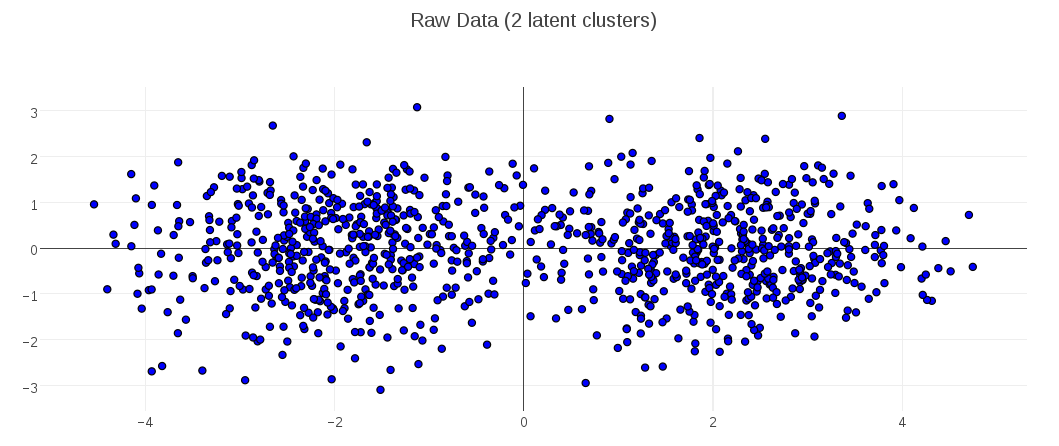
Consider this synthetic data set of points in 2D space. You can see that I’ve generated the data to have two latent clusters:
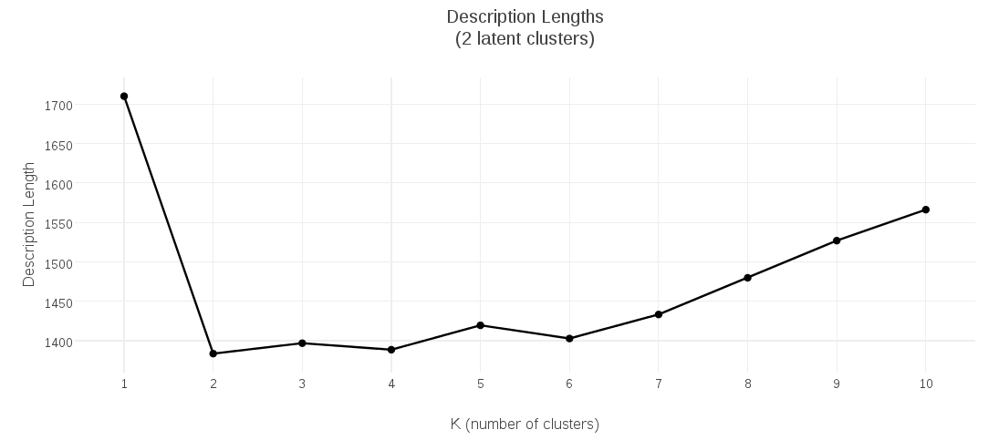
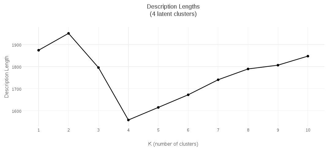
I collected the description-length values for candidate K-Medoids models having 1 up to 10 clusters, and plotted them. This plot shows that the clustering with minimal description length had 2 clusters:
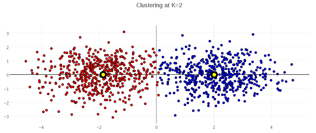
When I plot that optimal clustering at K=2 (with cluster medoids marked in black-and-yellow), the clustering looks good:
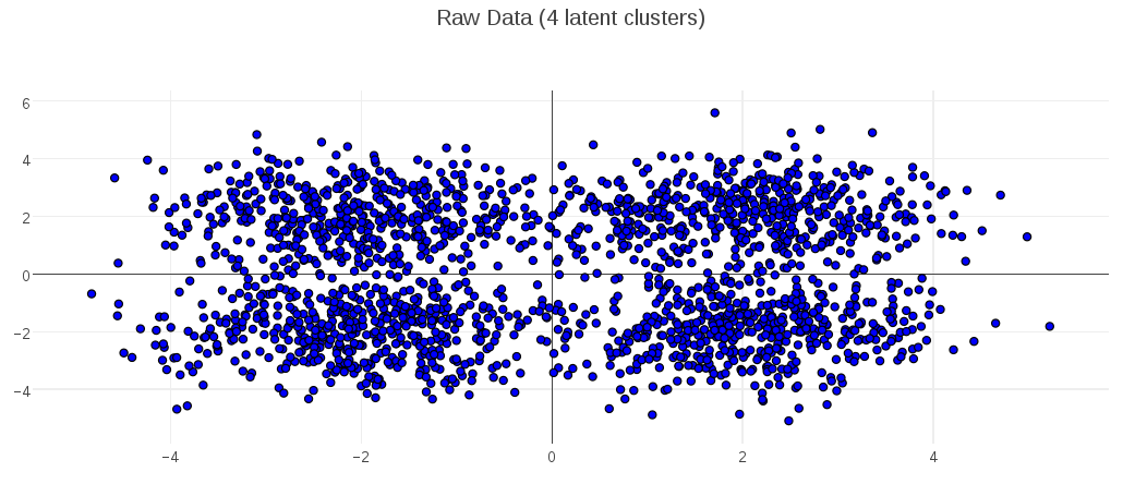
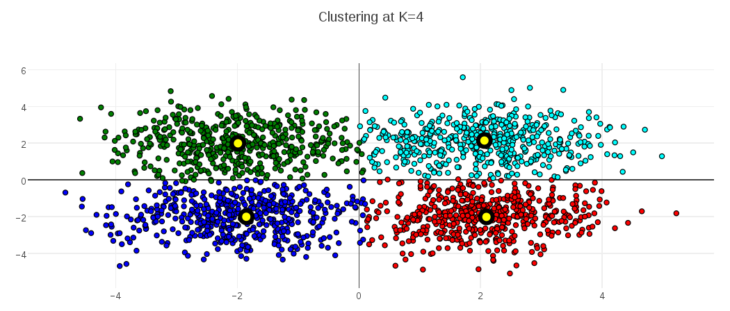
To show the behavior for a different optimal value, the following plots demonstrate the MDL K-Medoids results on data where the number of latent clusters is 4:
A final comment on Minimum Description Length approaches to clustering – although I focused on K-Medoids models in this post, the basic approach (and I suspect even the same description length formulation) would apply equally well to K-Means, and possibly other clustering models. Any clustering model that involves a distance function from elements to some kind of cluster center should be a good candidate. I intend to keep an eye out for applications of MDL to other learning models, as well.
References
[1] “Novelty Detection Using Extreme Value Statistics”; Stephen J. Roberts; Feb 23, 1999
[2] “Learning the k in k-means. Advances in neural information processing systems”; Hamerly, G., & Elkan, C.; 2004