Measuring Decision Tree Split Quality with Test Statistic P-Values
When training a decision tree learning model (or an ensemble of such models) it is often nice to have a policy for deciding when a tree node can no longer be usefully split. There are a variety possibilities. For example, halting when node population size becomes smaller than some threshold is a simple and effective policy. Another approach is to halt when some measure of node purity fails to increase by some minimum threshold. The underlying concept is to have some measure of split quality, and to halt when no candidate split has sufficient quality.
In this post I am going to discuss some advantages to one of my favorite approaches to measuring split quality, which is to use a test statistic significance – aka “p-value” – of the null hypothesis that the left and right sub-populations are the same after the split. The idea is that if a split is of good quality, then it ought to have caused the sub-populations to the left and right of the split to be meaningfully different. That is to say: the null hypothesis (that they are the same) should be rejected with high confidence, i.e. a small p-value. What constitutes “small” is always context dependent, but popular p-values from applied statistics are 0.05, 0.01, 0.005, etc.
update – there is now an Apache Spark JIRA and a pull request for this feature
The remainder of this post is organized in the following sections:
Consistency
Awareness of Sample Sizes
Training Results
Conclusion
Consistency
Test statistic p-values have some appealing properties as a split quality measure. The test statistic methodology has the advantage of working essentially the same way regardless of the particular test being used. We begin with two sample populations; in our case, these are the left and right sub-populations created by a candidate split. We want to assess whether these two populations have the same distribution (the null hypothesis) or different distributions. We measure some test statistic ‘S’ (Student’s t, Chi-Squared, etc). We then compute the probability that \(\vert S \vert\) >= the value we actually measured. This probability is commonly referred to as the p-value. The smaller the p-value, the less likely it is that our two populations are the same. In our case, we can interpret this as: a smaller p-value indicates a better quality split.
This consistent methodology has a couple advantages contributing to user experience (UX). If all measures of split quality work in the same way, then there is a lower cognitive load to move between measures once the user understands the common pattern of use. A second advantage is better “unit analysis.” Since all such quality measures take the form of p-values, there is no risk of a chosen quality measure getting mis-aligned with a corresponding quality threshold. They are all probabilities, on the interval [0,1], and “smaller threshold” always means “higher threshold of split quality.” By way of comparison, if an application is measuring entropy and then switches to using Gini impurity, these measures are in differing units and care has to be taken that the correct quality threshold is used in each case or the model training policy will be broken. Switching between differing statistical tests does not come with the same risk. A p-value quality threshold will have the same semantic regardless of which statistical test is being applied: probability that left and right sub-populations are the same, given the particular statistic being measured.
Awareness of Sample Size
Test statistics have another appealing property: many are “aware” of sample size in a way that captures the idea that the smaller the sample size, the larger the difference between populations should be to conclude a given significance. For one example, consider Welch’s t-test, the two-sample variation of the t distribution that applies well to comparing left and right sub populations of candidate decision tree splits:
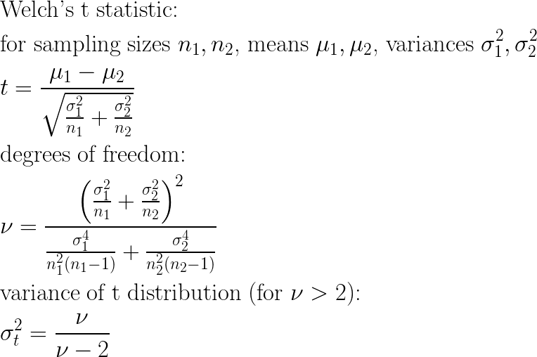
Visualizing the effects of sample sizes n1 and n2 on these equations directly is a bit tricky, but assuming equal sample sizes and variances allows the equations to be simplified quite a bit, so that we can observe the effect of sample size:
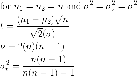
These simplified equations show clearly that (all else remaining equal) as sample size grows smaller, the measured t-statistic correspondingly grows smaller (proportional to sqrt(n)), and furthermore the corresponding variance of the t distribution to be applied grows larger. For any given shift in left and right sub-populations, each of these trends yields a larger (i.e. weaker) p-value. This behavior is desirable for a split quality metric. The less data there is at a given candidate split, the less confidence there should be in split quality. Put another way: we would like to require a larger difference before a split is measured as being good quality when we have less data to work with, and that is exactly the behavior the t-test provides us.
Training Results
These propreties are pleasing, but it remains to show that test statistics can actually improve decision tree training in practice. In the following sections I will compare the effects of training with test statstics with other split quality policies based on entropy and gini index.
To conduct these experiments, I modified a local copy of Apache Spark with the Chi-Squared test statistic for comparing categorical distributions. The demo script, which I ran in spark-shell, can be viewed here.
I generated an example data set that represents a two-class learning problem, where labels may be 0 or 1. Each sample has 10 clean binary features, such that if the bit is 1, the probability of the label is 90% 1 and 10% 0. There are 5 noise features, also binary, which are completely random. There are 50 samples of each clean feature being on, for a total of 500 samples. There are also 500 samples where all clean features are 0 and the corresponding labels are 90% 0 and 10% 1. The total number of samples in the data set is 1000. The shape of the data is illustrated by the following table:
truth |     features 0 - 9 (one on at a time)     |   random noise
------+-------------------------------------------+--------------
90% 1 | 1   0   0   0   0   0   0   0   0   0   0 | 1   0   0   1   0
90% 1 |  ... 50 samples with feature 0 'on' ...   |   ... noise ...
90% 1 | 0   1   0   0   0   0   0   0   0   0   0 | 0   1   1   0   0
90% 1 |  ... 50 samples with feature 1 'on' ...   |   ... noise ...
90% 1 |  ... 50 samples with feature 2 'on' ...   |   ... noise ...
90% 1 |  ... 50 samples with feature 3 'on' ...   |   ... noise ...
90% 1 |  ... 50 samples with feature 4 'on' ...   |   ... noise ...
90% 1 |  ... 50 samples with feature 5 'on' ...   |   ... noise ...
90% 1 |  ... 50 samples with feature 6 'on' ...   |   ... noise ...
90% 1 |  ... 50 samples with feature 7 'on' ...   |   ... noise ...
90% 1 |  ... 50 samples with feature 8 'on' ...   |   ... noise ...
90% 1 |  ... 50 samples with feature 9 'on' ...   |   ... noise ...
90% 0 | 0   0   0   0   0   0   0   0   0   0   0 | 1   1   0   0   1
90% 0 |  ... 500 samples with all 'off  ...       |   ... noise ...
For the first run I use my customized chi-squared statistic as the split quality measure. I used a p-value threshold of 0.01 – that is, I would like my chi-squared test to conclude that the probability of left and right split populations are the same is <= 0.01, or that split will not be used. Note, this means I can expect that around 1% of the time, it will conclude a split was good, when it was just luck. This is a reasonable false-positive rate; random forests are by nature robust to noise, including noise in their own split decisions:
scala> :load pval_demo
Loading pval_demo...
defined module demo

scala> val rf = demo.train("chisquared", 0.01, noise = 0.1)
  pval= 1.578e-09
gain= 20.2669
  pval= 1.578e-09
gain= 20.2669
  pval= 1.578e-09
gain= 20.2669
  pval= 9.140e-09
gain= 18.5106

... more tree p-value demo output ...

  pval= 0.7429
gain= 0.2971
  pval= 0.9287
gain= 0.0740
  pval= 0.2699
gain= 1.3096
rf: org.apache.spark.mllib.tree.model.RandomForestModel =
TreeEnsembleModel classifier with 1 trees


scala> println(rf.trees(0).toDebugString)
DecisionTreeModel classifier of depth 10 with 21 nodes
  If (feature 5 in {1.0})
   Predict: 1.0
  Else (feature 5 not in {1.0})
   If (feature 6 in {1.0})
    Predict: 1.0
   Else (feature 6 not in {1.0})
    If (feature 0 in {1.0})
     Predict: 1.0
    Else (feature 0 not in {1.0})
     If (feature 1 in {1.0})
      Predict: 1.0
     Else (feature 1 not in {1.0})
      If (feature 2 in {1.0})
       Predict: 1.0
      Else (feature 2 not in {1.0})
       If (feature 8 in {1.0})
        Predict: 1.0
       Else (feature 8 not in {1.0})
        If (feature 3 in {1.0})
         Predict: 1.0
        Else (feature 3 not in {1.0})
         If (feature 4 in {1.0})
          Predict: 1.0
         Else (feature 4 not in {1.0})
          If (feature 7 in {1.0})
           Predict: 1.0
          Else (feature 7 not in {1.0})
           If (feature 9 in {1.0})
            Predict: 1.0
           Else (feature 9 not in {1.0})
            Predict: 0.0

scala>
The first thing to observe is that the resulting decision tree used exactly the 10 clean features 0 through 9, and none of the five noise features. The tree splits off each of the clean features to obtain an optimally accurate leaf-node (one with 90% 1s and 10% 0s). A second observation is that the p-values shown in the demo output are extremely small (i.e. strong) values – around 1e-9 (one part in a billion) – for good-quality splits. We can also see “weak” p-values with magnitudes such as 0.7, 0.2, etc. These are poor quality splits on the noise features that it rejects and does not use in the tree, exactly as we hope to see.
Next, I will show a similar run with the standard available “entropy” quality measure, and a minimum gain threshold of 0.035, which is a value I had to determine by trial and error, as what kind of entropy gains one can expect to see, and where to cut them off, is somewhat unintuitive and likely to be very data dependent.
scala> val rf = demo.train("entropy", 0.035, noise = 0.1)
  impurity parent= 0.9970, left= 0.3274 (  50), right= 0.9997 ( 950) weighted= 0.9661
gain= 0.0310
  impurity parent= 0.9970, left= 0.1414 (  50), right= 0.9998 ( 950) weighted= 0.9569
gain= 0.0402
  impurity parent= 0.9970, left= 0.3274 (  50), right= 0.9997 ( 950) weighted= 0.9661
gain= 0.0310

... more demo output ...

rf: org.apache.spark.mllib.tree.model.RandomForestModel =
TreeEnsembleModel classifier with 1 trees


scala> println(rf.trees(0).toDebugString)
DecisionTreeModel classifier of depth 11 with 41 nodes
  If (feature 4 in {1.0})
   If (feature 12 in {1.0})
    If (feature 11 in {1.0})
     Predict: 1.0
    Else (feature 11 not in {1.0})
     Predict: 1.0
   Else (feature 12 not in {1.0})
    Predict: 1.0
  Else (feature 4 not in {1.0})
   If (feature 1 in {1.0})
    If (feature 12 in {1.0})
     Predict: 1.0
    Else (feature 12 not in {1.0})
     Predict: 1.0
   Else (feature 1 not in {1.0})
    If (feature 0 in {1.0})
     If (feature 10 in {0.0})
      If (feature 14 in {1.0})
       Predict: 1.0
      Else (feature 14 not in {1.0})
       Predict: 1.0
     Else (feature 10 not in {0.0})
      If (feature 14 in {0.0})
       Predict: 1.0
      Else (feature 14 not in {0.0})
       Predict: 1.0
    Else (feature 0 not in {1.0})
     If (feature 6 in {1.0})
      Predict: 1.0
     Else (feature 6 not in {1.0})
      If (feature 3 in {1.0})
       Predict: 1.0
      Else (feature 3 not in {1.0})
       If (feature 7 in {1.0})
        If (feature 13 in {1.0})
         Predict: 1.0
        Else (feature 13 not in {1.0})
         Predict: 1.0
       Else (feature 7 not in {1.0})
        If (feature 2 in {1.0})
         Predict: 1.0
        Else (feature 2 not in {1.0})
         If (feature 8 in {1.0})
          Predict: 1.0
         Else (feature 8 not in {1.0})
          If (feature 9 in {1.0})
           If (feature 11 in {1.0})
            If (feature 13 in {1.0})
             Predict: 1.0
            Else (feature 13 not in {1.0})
             Predict: 1.0
           Else (feature 11 not in {1.0})
            If (feature 12 in {1.0})
             Predict: 1.0
            Else (feature 12 not in {1.0})
             Predict: 1.0
          Else (feature 9 not in {1.0})
           If (feature 5 in {1.0})
            Predict: 1.0
           Else (feature 5 not in {1.0})
            Predict: 0.0

scala>
The first observation is that the resulting tree using entropy as a split quality measure is twice the size of the tree trained using the chi-squared policy. Worse, it is using the noise features – its quality measure is yielding many more false positives. The entropy-based model is less parsimonious and will also have performance problems since the model has included very noisy features.
Lastly, I ran a similar training using the “gini” impurity measure, and a 0.015 quality threshold (again, hopefully optimal value that I had to run multiple experiments to identify). Its quality is better than the entropy-based measure, but this model is still substantially larger than the chi-squared model, and it still uses some noise features:
scala> val rf = demo.train("gini", 0.015, noise = 0.1)
  impurity parent= 0.4999, left= 0.2952 (  50), right= 0.4987 ( 950) weighted= 0.4885
gain= 0.0113
  impurity parent= 0.4999, left= 0.2112 (  50), right= 0.4984 ( 950) weighted= 0.4840
gain= 0.0158
  impurity parent= 0.4999, left= 0.1472 (  50), right= 0.4981 ( 950) weighted= 0.4806
gain= 0.0193
  impurity parent= 0.4999, left= 0.2112 (  50), right= 0.4984 ( 950) weighted= 0.4840
gain= 0.0158

... more demo output ...

rf: org.apache.spark.mllib.tree.model.RandomForestModel =
TreeEnsembleModel classifier with 1 trees

scala> println(rf.trees(0).toDebugString)
DecisionTreeModel classifier of depth 12 with 31 nodes
  If (feature 6 in {1.0})
   Predict: 1.0
  Else (feature 6 not in {1.0})
   If (feature 3 in {1.0})
    Predict: 1.0
   Else (feature 3 not in {1.0})
    If (feature 1 in {1.0})
     Predict: 1.0
    Else (feature 1 not in {1.0})
     If (feature 8 in {1.0})
      Predict: 1.0
     Else (feature 8 not in {1.0})
      If (feature 2 in {1.0})
       If (feature 14 in {0.0})
        Predict: 1.0
       Else (feature 14 not in {0.0})
        Predict: 1.0
      Else (feature 2 not in {1.0})
       If (feature 5 in {1.0})
        Predict: 1.0
       Else (feature 5 not in {1.0})
        If (feature 7 in {1.0})
         Predict: 1.0
        Else (feature 7 not in {1.0})
         If (feature 0 in {1.0})
          If (feature 12 in {1.0})
           If (feature 10 in {0.0})
            Predict: 1.0
           Else (feature 10 not in {0.0})
            Predict: 1.0
          Else (feature 12 not in {1.0})
           Predict: 1.0
         Else (feature 0 not in {1.0})
          If (feature 9 in {1.0})
           Predict: 1.0
          Else (feature 9 not in {1.0})
           If (feature 4 in {1.0})
            If (feature 10 in {0.0})
             Predict: 1.0
            Else (feature 10 not in {0.0})
             If (feature 14 in {0.0})
              Predict: 1.0
             Else (feature 14 not in {0.0})
              Predict: 1.0
           Else (feature 4 not in {1.0})
            Predict: 0.0

scala>
Conclusion
In this post I have discussed some advantages of using test statstics and p-values as split quality metrics for decision tree training:
- Consistency
- Awareness of sample size
- Higher quality model training
I believe they are a useful tool for improved training of decision tree models! Happy computing!