Random Forest Clustering of Machine Package Configurations in Apache Spark
In this post I am going to describe some results I obtained for clustering machines by which RPM packages that were installed on them. The clustering technique I used was Random Forest Clustering.
The Data
The data I clustered consisted of 135 machines, each with a list of installed RPM packages. The number of unique package names among all 135 machines was 4397. Each machine was assigned a vector of Boolean values: a value of 1 indicates that the corresponding RPM was installed on that machine. This means that the clustering data occupied a space of nearly 4400 dimensions. I discuss the implications of this later in the post, and what it has to do with Random Forest Clustering in particular.
For ease of navigation and digestion, the remainder of this post is organized in sections:
Introduction to Random Forest Clustering
(The Pay-Off)
Package Configuration Clustering Code
Clustering Results
(Outliers)
Random Forests and Random Forest Clustering
Full explainations of Random Forests and Random Forest Clustering could easily occupy blog posts of their own, but I will attempt to summarize them briefly here. Random Forest learning models per se are well covered in the machine learning community, and available in most machine learning toolkits. With that in mind, I will focus on their application to Random Forest Clustering, as it is less commonly used.
A Random Forest is an ensemble learning model, consisting of some number of individual decision trees, each trained on a random subset of the training data, and which choose from a random subset of candidate features when learning each internal decision node.
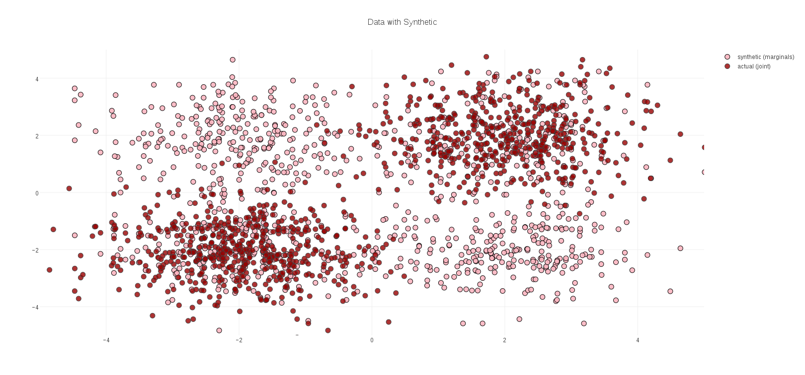
Random Forest Clustering begins by training a Random Forest to distinguish between the data to be clustered, and a corresponding synthetic data set created by sampling from the marginal distributions of each feature. If the data has well defined clusters in the joint feature space (a common scenario), then the model can identify these clusters as standing out from the more homogeneous distribution of synthetic data. A simple example of what this looks like in 2 dimensional data is displayed in Figure 1, where the dark red dots are the data to be clustered, and the lighter pink dots represent synthetic data generated from the marginal distributions:
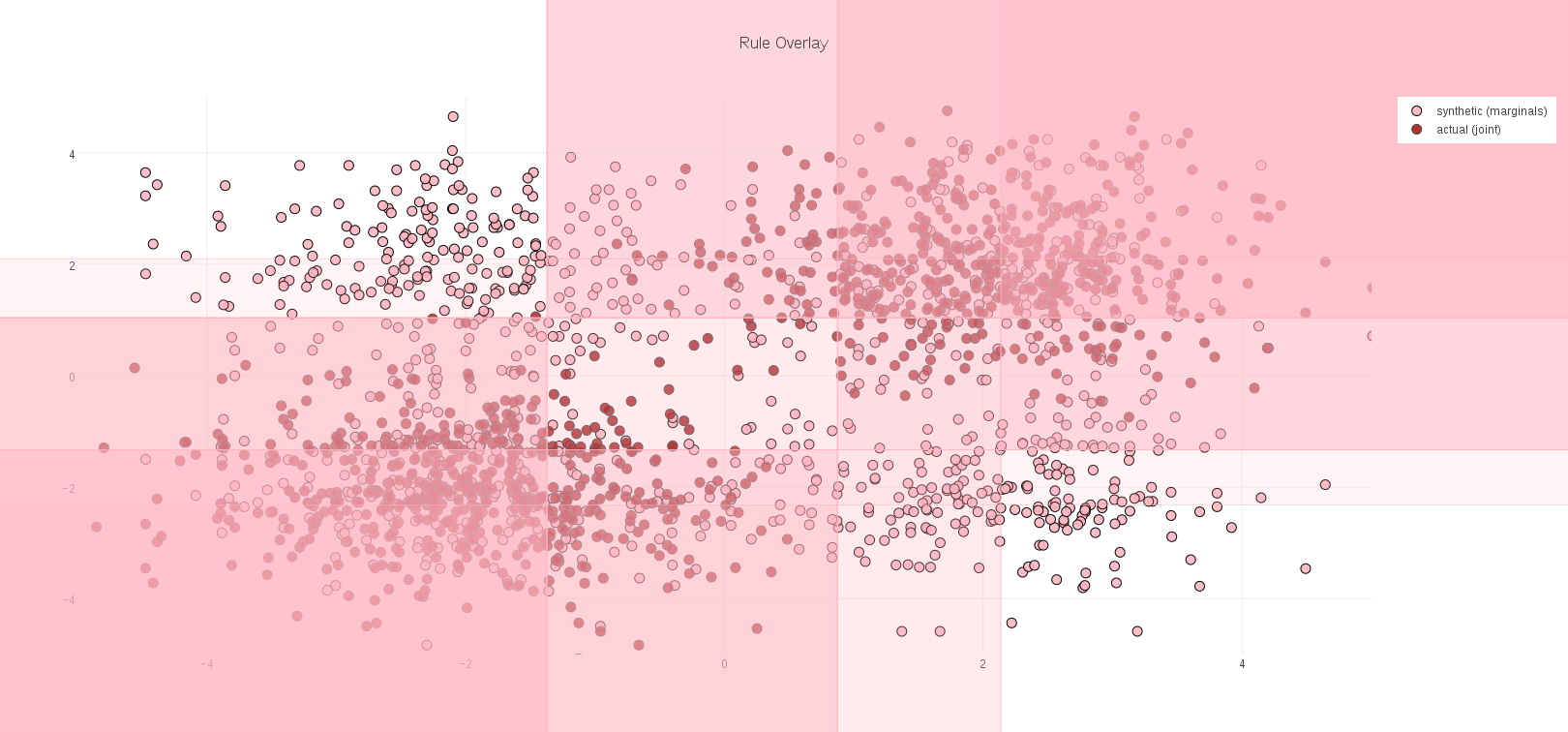
Each interior decision node, in each tree of a Random Forest, typically divides the space of feature vectors in half: the half-space <= some threshold, and the half-space > that threshold. The result is that the model learned for our data can be visualized as rectilinear regions of space. In this simple example, these regions can be plotted directly over the data, and show that the Random Forest did indeed learn the location of the data clusters against the background of synthetic data:
Once this model has been trained, the actual data to be clustered are evaluated against this model. Each data element navigates the interior decision nodes and eventually arrives at a leaf-node of each tree in the Random Forest ensemble, as illustrated in the following schematic:
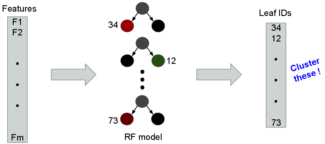
A key insight of Random Forest Clustering is that if two objects (or, their feature vectors) are similar, then they are likely to arrive at the same leaf nodes more often than not. As the figure above suggests, it means we can cluster objects by their corresponding vectors of leaf nodes, instead of their raw feature vectors.
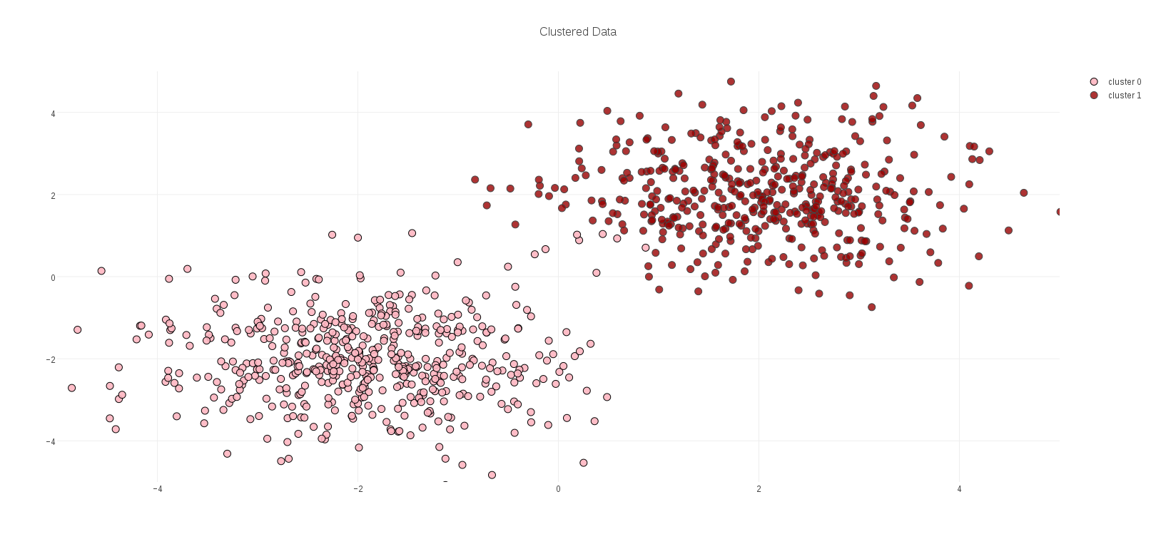
If we map the points in our toy example to leaf ids in this way, and then cluster the results, we obtain the following two clusters, which correspond well with the structure of the data:
A note on clustering leaf ids. A leaf id is just that – an identifier – and in that respect a vector of leaf ids has no algebra; it is not meaningful to take an average of such identifiers, any more than it would be meaningful to take the average of people’s names. Pragmatically, what this means is that the popular k-means clustering algorithm cannot be applied to this problem.
These vectors do, however, have distance: for any pair of vectors, add 1 for each corresponding pair of leaf ids that differ. If two data elements arrived at all the same leafs in the Random Forest model, all their leaf ids are the same, and their distance is zero (with respect to the model, they are the same). Therefore, we can apply k-medoids clustering.
The Pay-Off
What does this somewhat indirect method of clustering buy us? Why not just cluster objects by their raw feature vectors?
The problem is that in many real-world cases (unlike in our toy example above), feature vectors computed for objects have many dimensions – hundreds, thousands, perhaps millions – instead of the two dimensions in this example. Computing distances on such objects, necessary for clustering, is often expensive, and worse yet the quality of these distances is frequently poor due to the fact that most features in large spaces will be poorly correlated with any structure in the data. This problem is so common, and so important, it has a name: the Curse of Dimensionality.
Random Forest Clustering, which clusters on vectors of leaf-node ids from the trees in the model, side-steps the curse of dimensionality because the Random Forest training process, by learning where the data is against the background of the synthetic data, has already identified the features that are useful for identifying the structure of the data! If any particular feature was poorly correlated with that struture, it has already been ignored by the model. In other words, a Random Forest Clustering model is implicitly examining ** exactly those features that are most useful for clustering **, thus providing a cure for the Curse of Dimensionality.
The machine package configurations whose clustering I describe for this post are a good example of high dimensional data that is vulnerable to the Curse of Dimensionality. The dimensionality of the feature space is nearly 4400, making distances between vectors potentially expensive to evaluate. Any individual feature contributes little to the distance, having to contend with over 4000 other features. Installed packages are also noisy. Many packages, such as kernels, are installed everywhere. Others may be installed but not used, making them potentially irrelevant to grouping machines. Furthermore, there are only 135 machines, and so there are far more features than data examples, making this an underdetermined data set.
All of these factors make the machine package configuration data a good test of the strenghts of Random Forest Clustering.
Package Configuration Clustering Code
The implementation of Random Forest Clustering I used for the results in this post is a library available from the silex project, a package of analytics libraries and utilities for Apache Spark.
In this section I will describe three code fragments that load the machine configuration data, perform a Random Forest clustering, and format some of the output. This is the code I ran to obtain the results described in the final section of this post.
The first fragment of code illustrates the logistics of loading the feature vectors from file train.txt that represent the installed-package configurations for each machine. A corresponding “parallel” file nodesclean.txt contains corresponding machine names for each vector. A third companion file rpms.txt contains names of each installed package. These are used to instantiate a specialized Scala function (InvertibleIndexFunction) between feature indexes and human-readable feature names (in this case, names of RPM packages). Finally, another specialized function (Extractor) for instantiating Spark feature vectors is created.
Note: Extractor and InvertibleIndexFunction are also component libraries of silex
// Load installed-package feature vectors
val fields = spark.textFile(s"$dataDir/train.txt").map(_.split(" ").toVector)

// Pair feature vectors with machine names
val nodes = spark.textFile(s"$dataDir/nodesclean.txt").map { _.split(" ")(1) }
val ids = fields.paste(nodes)

// Load map from feature indexes to package names
val inp = spark.textFile(s"$dataDir/rpms.txt").map(_.split(" "))
  .map(r => (r(0).toInt, r(1)))
  .collect.toVector.sorted
val nf = InvertibleIndexFunction(inp.map(_._2))

// A feature extractor maps features into sequence of doubles
val m = fields.first.length - 1
val ext = Extractor(m, (v: Vector[String]) => v.map(_.toDouble).tail :FeatureSeq)
  .withNames(nf)
  .withCategoryInfo(IndexFunction.constant(2, m))
The next section of code is where the work of Random Forest Clustering happens. A RandomForestCluster object is instantiated, and configured. Here, the configuration is for 7 clusters, 250 synthetic points (about twice as many synthetic points as true data), and a Random Forest of 20 trees. Training against the input data is a simple call to the run method.
The predictWithDistanceBy method is then applied to the data paired with machine names, to yield tuples of cluster-id, distance to cluster center, and the associated machine name. These tuples are split by distance into data with a cluster, and data considered to be “outliers” (i.e. elements far from any cluster center). Lastly, the histFeatures method is applied, to examine the Random Forest Model and identify any commonly-used features.
// Train a Random Forest Clustering Model
val rfcModel = RandomForestCluster(ext)
  .setClusterK(7)
  .setSyntheticSS(250)
  .setRfNumTrees(20)
  .setSeed(37)
  .run(fields)

// Evaluate to get tuples: (cluster, distance, machine-name)
val cid = ids.map(rfcModel.predictWithDistanceBy(_)(x => x))

// Split by closest distances into clusters and outliers
val (clusters, outliers) = cid.splitFilter { case (_, dist, _) => dist <= 5 }

// Generate a histogram of features used in the RF model
val featureHist = rfcModel.randomForestModel.histFeatures(ext.names)
The final code fragment simply formats clusters and outliers into a tabular form, as displayed in the next section of this post. Note that there is neither Spark nor silex code here; standard Scala methods are sufficient to post-process the clustering data:
// Format clusters for display
val clusterStr = clusters.map { case (j, d, n) => (j, (d, n)) }
  .groupByKey
  .collect
  .map { case (j, nodes) =>
    nodes.toSeq.sorted.map { case (d, n) => s"$d  $n" }.mkString("\n")
  }
  .mkString("\n\n")

// Format outliers for display
val outlierStr = outliers.collect
  .map { case (_, d,n) => (d, n) }
  .toVector.sorted
  .map { case (d, n) => s"$d  $n" }
  .mkString("\n")
Package Configuration Clustering Results
The result of running the code in the previous section is seven clusters of machines. In the following files, the first column represents distance from the cluster center, and the second is the actual machine’s node name. A cluster distance of 0.0 indicates that the machine was indistinguishable from cluster center, as far as the Random Forest model was concerned. The larger the distance, the more different from the cluster’s center a machine was, in terms of its installed RPM packages.
Was the clustering meaningful? Examining the first two clusters below is promising; the machine names in these clusters are clearly similar, likely configured for some common task by the IT department. The first cluster of machines appears to be web servers and corresponding backend services. It would be unsurprising to find their RPM configurations were similar.
The second cluster is a series of executor machines of varying sizes, but presumably these would be configured similarly to one another.
The second pair of clusters (3 & 4) are small. All of their names are similar (and furthermore, similar to some machines in other clusters), and so an IT administrator might wonder why they ended up in oddball small clusters. Perhaps they have some spurious, non-standard packages installed that ought to be cleaned up. Identifying these kinds of structure in a clustering is one common clustering application.
Cluster 5 is a series of bugzilla web servers and corresponding back-end bugzilla data base services. Although they were clustered together, we see that the web servers have a larger distance from the center, indicating a somewhat different configuration.
Cluster 6 represents a group of performance-related machines. Not all of these machines occupy the same distance, even though most of their names are similar. These are also the same series of machines as in clusters 3 & 4. Does this indicate spurious package installations, or some other legitimate configuration difference? A question for the IT department…
Cluster 7 is by far the largest. It is primarily a combination of OpenStack machines and yet more perf machines. This clustering was relatively stable – it appeared across multiple independent clustering runs. Because of its stability I would suggest to an IT administrator that the performance and OpenStack machines are sharing some configuration similarities, and the performance machines in other clusters suggest that there might be yet more configuration anomalies. Perhaps these were OpenStack nodes that were re-purposed as performance machines? Yet another question for IT…
Outliers
This last grouping represents machines which were “far” from any of the previous cluster centers. They may be interpreted as “outliers” - machines that don’t fit any model category. Of these the node frodo is clearly somebody’s personal machine, likely with a customized or idiosyncratic package configuration. Unsurprising that it is farthest of all machines from any cluster, with distance 9.0. The jenkins machine is also somewhat unique among the nodes, and so perhaps not surprising that its registers as anomalous. The remaining machines match node series from other clusters. Their large distance is another indication of spurious configurations for IT to examine.
I will conclude with another useful feature of Random Forest Models, which is that you can interrogate them for information such as which features were used most frequently. Here is a histogram of model features (in this case, installed packages) that were used most frequently in the clustering model. This particular histogram i sinteresting, as no feature was used more than twice. The remaining features were all used exactly once. This is a bit unusual for a Random Forest model. Frequently some features are used commonly, with a longer tail. This histogram is rather “flat,” which may be a consequence of there being many more features (over 4000 installed packages) than there are data elements (135 machines). This makes the problem somewhat under-determined. To its credit, the model still achieves a meaningful clustering.
Lastly I’ll note that full histogram length was 186; in other words, of the nearly 4400 installed packages, the Random Forest model used only 186 of them – a tiny fraction! A nice illustration of Random Forest Clustering performing in the face of high dimensionality!