Parallel K-Medoids Using Scala ParSeq
Scala supplies a parallel collections library that was designed to make it easy for a programmer to add parallel computing over the elements in a collection. In this post, I will describe a case study of applying Scala’s parallel collections to cleanly implement multithreading support for training a K-Medoids clustering model.
Motivation
K-Medoids clustering is a relative of K-Means clustering that does not require an algebra over input data elements. That is, K-Medoids requires only a distance metric defined on elements in the data space, and can cluster objects which do not have a well-defined concept of addition or division that is necessary for computing the centroids required by K-Means. For example, K-Medoids can cluster character strings, which have a notion of distance, but no notion of summation that could be used to compute a geometric centroid.
This additional generality comes at a cost. The medoid of a collection of elements is the member of the collection that minimizes some function F of the distances from that element to all the other elements in the collection. For example, F might be the sum of distances from one element to all the elements, or perhaps the maximum distance, etc. It is not hard to see that the cost of computing a medoid of (n) elements is quadratic in (n): Evaluating F is linear in (n) and F in turn must be evaluated with respect to each element. Furthermore, unlike centroid-based computations used in K-Means, computing a medoid does not naturally lend itself to common scale-out computing formalisms such as Spark RDDs, due to the full-cross-product nature of the computation.
With this in mind, a more traditional multithreading approach is a good candidate to achieve some practical parallelism on modern multi-core hardware. I’ll demonstrate that this is easy to implement in Scala with parallel sequences.
Non-Parallel Code
Consider a baseline non-parallel implementation of K-Medoids, as in the following example skeleton code. (A working version of this code, under review at the time of this post, can be viewed here)
class KMedoids[T](k: Int, metric: (T, T) => Double) {

  // Train a K-Medoids cluster on some input data
  def train[T](data: Seq[T]) {
    var current = // randomly select k data elements as initial cluster

    var model_converged = false
    while (!model_converged) {
      // assign each element to its closest medoid
      val clusters = data.groupBy(medoidIdx(_, current)).map(_._2)

      // recompute the medoid from the latest cluster elements
      val next = benchmark("medoids") {
        clusters.map(medoid)
      }

      model_converged = // test for model convergence

      current = next
    }
  }

  // Return the medoid of some collection of elements
  def medoid(data: Seq[T]) = {
    benchmark(s"medoid: n= ${data.length}") {
      data.minBy(medoidCost(_, data)
    }
  }

  // The sum of an element's distance to all the elements in its cluster
  def medoidCost(e: T, data: Seq[T]) = data.iterator.map(metric(e, _)).sum

  // Index of the closest medoid to an element
  def medoidIdx(e: T, mv: Seq[T]) = mv.iterator.map(metric(e, _)).zipWithIndex.min._2

  // Output a benchmark timing of some expression
  def benchmark[T](label: String)(blk: => T) = {
    val t0 = System.nanoTime
    val t = blk
    val sec = (System.nanoTime - t0) / 1e9
    println(f"Run time for $label = $sec%.1f"); System.out.flush
    t
  }
}
If we run the code above (de-skeletonized), then we might see something like this output from our benchmarking, where I clustered a dataset of 40,000 randomly-generated (x,y,z) points by Gaussian sampling around 5 chosen centers. (This data is numeric, but I provide only a distance metric on the points. K-Medoids has no knowledge of the data except that it can run the given metric function on it):
Run time for medoid: n= 8299 = 7.7
Run time for medoid: n= 3428 = 1.2
Run time for medoid: n= 12581 = 17.0
Run time for medoid: n= 5731 = 3.3
Run time for medoid: n= 9961 = 10.2
Run time for medoids = 39.8
Observe that cluster sizes are generally not the same, and we can see the time per cluster varying quadratically with respect to cluster size.
A First Take On Parallel K-Medoids
Studying our non-parallel code above, we can see that the computation of each new medoid is independent, which makes it a likely place to inject some parallelism. A Scala sequence can be transformed into a corresponding parallel sequence using the par method, and so parallelizing our code is literally this simple:
      // recompute the medoid from the latest cluster elements
      val next = benchmark("medoids") {
        clusters.par.map(medoid).seq
      }
In this block, I also apply .seq at the end, which is not always necessary but can avoid type mismatches between Seq[T] and ParSeq[T] under some circumstances.
In my case I also wish to exercise some control over the threading used by the parallelism, and so I explicitly assign a ForkJoinPool thread pool to the sequence:
      // establish a thread pool for use by K-Medoids
      val threadPool = new ForkJoinPool(numThreads)

      // ...

      // recompute the medoid from the latest cluster elements
      val next = benchmark("medoids") {
        val pseq = clusters.par
        pseq.tasksupport = new ForkJoinTaskSupport(threadPool)
        pseq.map(medoid).seq
      }
Minor grievance: it would be nice if Scala supported some ‘in-line’ methods, like seq.par(n)... and seq.par(threadPool)..., instead of requiring the programmer to break the flow of the code to invoke tasksupport =, which returns Unit.
Now that we’ve parallelized our K-Medoids training, we should see how well it responds to additional threads. I ran the above parallelized version using {1, 2, 4, 8, 16, 32} threads, on a machine with 40 cores, so that my benchmarking would not be impacted by attempting to run more threads than there are cores to support them. I also ran two versions of test data. The first I generated with clusters of equal size (5 clusters of ~8000 elements), and the second with one cluster being twice as large (1 cluster of ~13300 and 4 clusters of ~6700). Following is a plot of throughput (iterations / second) versus threads:
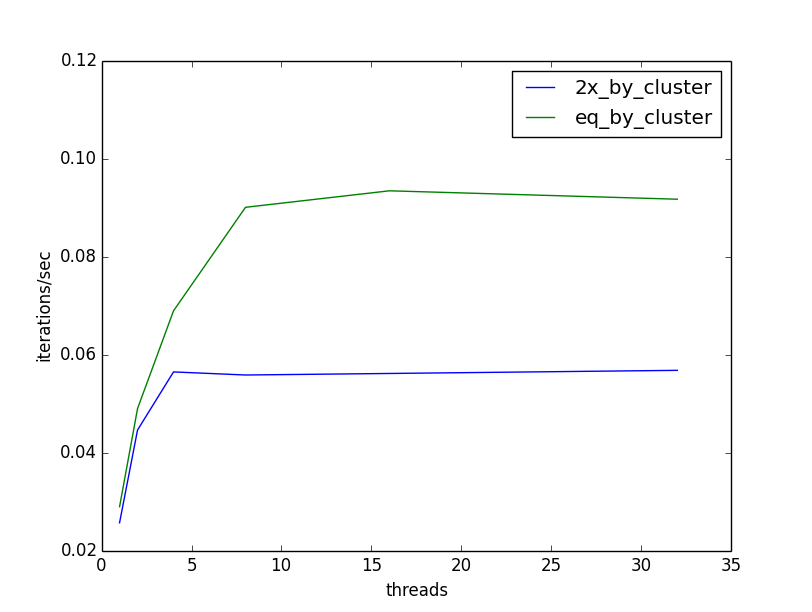
In the best of all possible worlds, our throughput would increase linearly with the number of threads; double the threads, double our iterations per second. Instead, our throughput starts to increase nicely as we add threads, but hits a hard ceiling at 8 threads. It is not hard to see why: our parallelism is limited by the number of elements in our collection of clusters. In our case that is k = 5, and so we reach our ceiling at 8 threads, the first thread number >= 5. Furthermore, we see that when the size of clusters is unequal, the throughput suffers even more. The time required to complete the clustering is dominated by the most expensive element. In our case, the cluster that is twice the size of other clusters:
Run time for medoid: n= 6695 = 5.1
Run time for medoid: n= 6686 = 5.2
Run time for medoid: n= 6776 = 5.3
Run time for medoid: n= 6682 = 5.4
Run time for medoid: n= 13161 = 19.9
Run time for medoids = 19.9
Take 2: Improving The Use Of Threads
Fortunately it is not hard to improve on this situation. If parallelizing by cluster is too coarse, we can try pushing our parallelism down one level of granularity. In our case, that means parallelizing the outer loop of our medoid function, and it is just as easy as before:
  // Return the medoid of some collection of elements
  def medoid(data: Seq[T]) = {
    benchmark(s"medoid: n= ${data.length}") {
      val pseq = data.par
      pseq.tasksupport = new ForkJoinTaskSupport(threadPool)
      pseq.minBy(medoidCost(_, data)
    }
  }
Note that I retained the previous parallelism at the cluster level, otherwise the algorithm would execute parallel medoids, but one cluster at a time. Also observe that we are applying the same thread pool we supplied to the ParSeq at the cluster level. Scala’s parallel logic can utilize the same thread pool at multiple granularities without blocking. This makes it very clean to control the total number of threads used by some computation, by simply re-using the same threadpool across all points of parallelism.
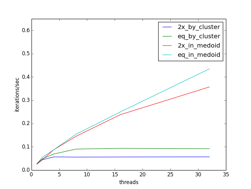
Now, when we re-run our experiment, we see that our throughput continues to increase as we add threads. The following plot illustrates the throughput increasing in comparison to the previous ceiling, and also that throughput is less sensitive to the cluster size, as threads can be allocated flexibly across clusters as they are available:
I hope this short case study has demonstrated how easy it is to add multithreading to computations with Scala parallel sequences, and some considerations for making the best use of available threads. Happy Parallel Programming!