Examining the Modulus of Random Variables
Motivation
The original motivation for these experiments was consideration of the impact of negotiator cycle cadence (i.e. the time between the start of one cycle and the start of the next) on HTCondor pool loading. Specifically, any HTCondor job that completes and vacates its resource may leave that resource unloaded until it can be re-matched on the next cycle. Therefore, the duration of resource vacancies (and hence, pool loading) can be thought of as a function of job durations modulo the cadence of the negotiator cycle. In general, the aggregate behavior of job durations on a pool is useful to model as a random variable. And so, it seemed worthwhile to build up a little intuition about the behavior of a random variable when you take its modulus.
Methodology
I took a Monte Carlo approach to this study because a tractable theoretical framework eluded me, and you do not have to dive very deep to show that even trivial random variable behavior under a modulus is dependent on the distribution. A Monte Carlo framework for the study also allows for other underlying distributions to be easily studied, by altering the random variable being sampled. In the interest of getting right into results, I’ll briefly discuss the tools I used at the end of this post.
Modulus and Variance
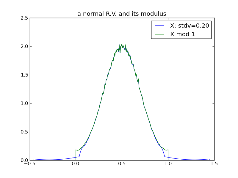
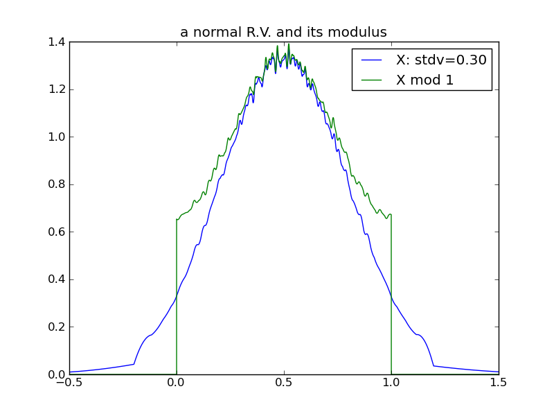
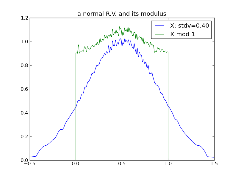
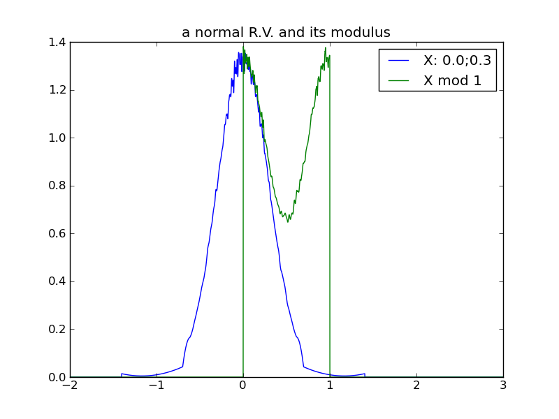
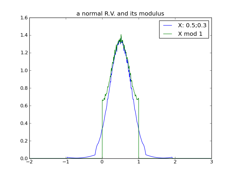
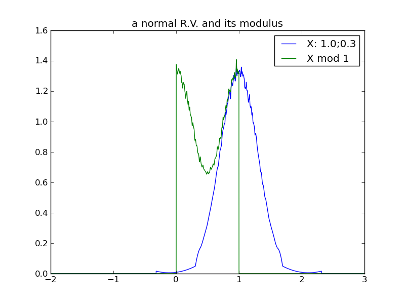
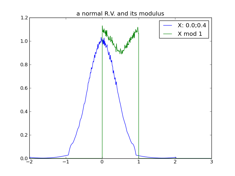
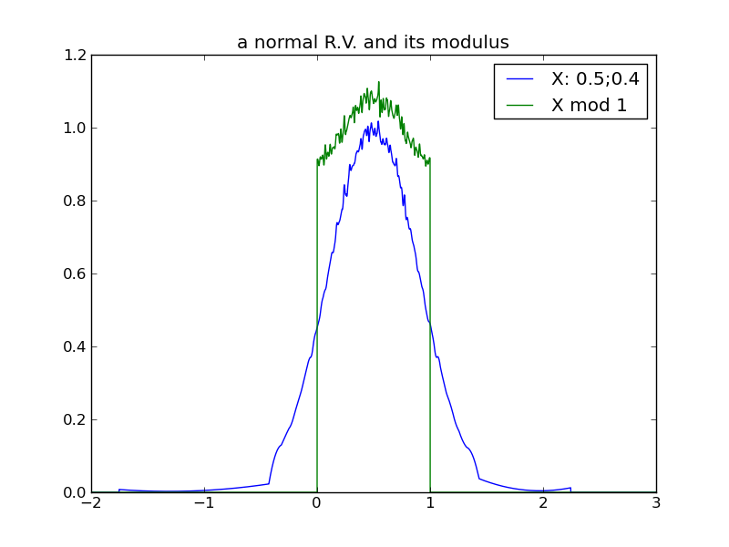
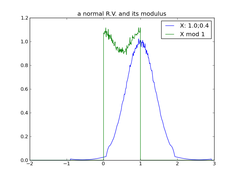
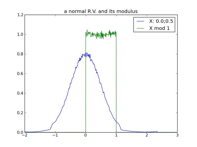
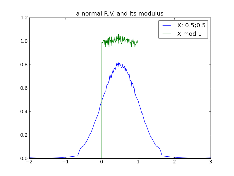
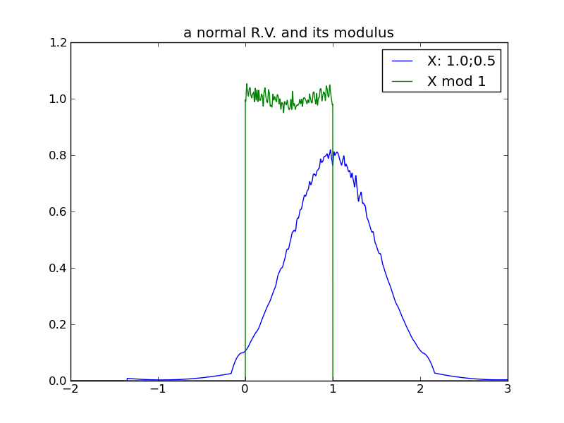
Consider what happens to a random variable’s modulus as its variance increases. This sequence of plots shows that the modulus of a normal distribution tends toward a uniform distribution over the modulus interval, as the underlying variance increases:
 |
 |
 |
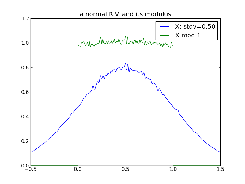 |
From the above plots, we can see that in the case of a normal distribution, its modulus tends toward uniform rather quickly - by the time the underlying variance is half of the modulus interval.
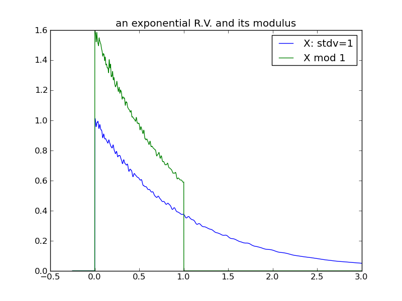
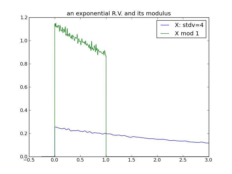
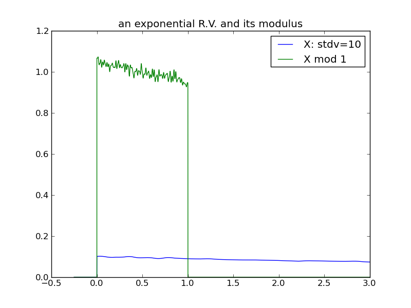
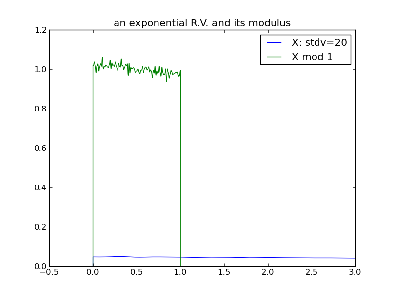
The following plots demonstrate the same effect with a one-tailed distribution (the exponential) – it requires a larger variance for the effect to manifest.
 |
 |
 |
 |
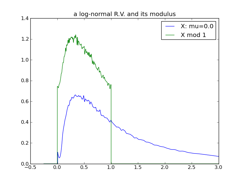
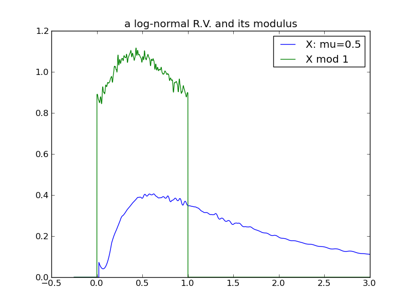
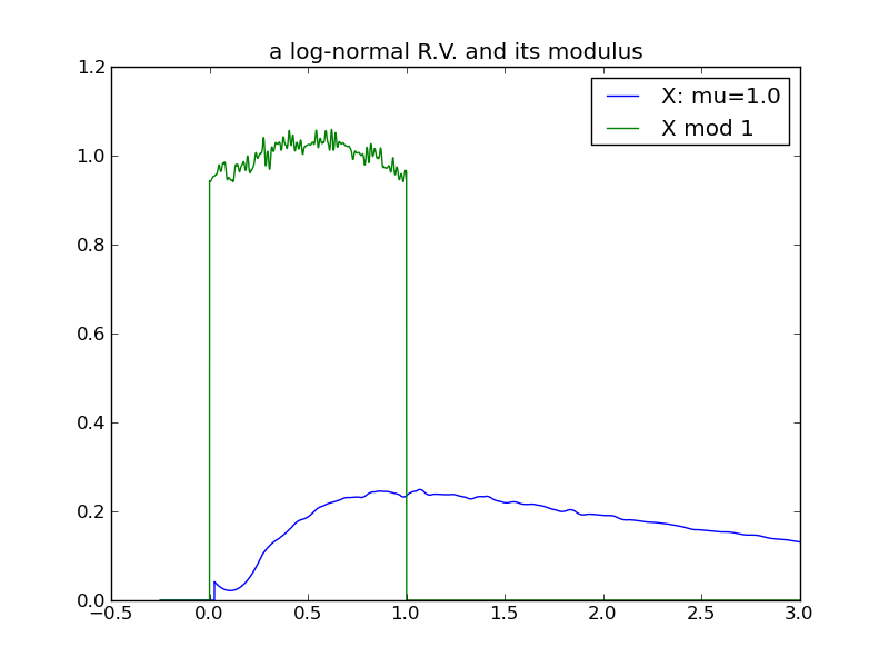
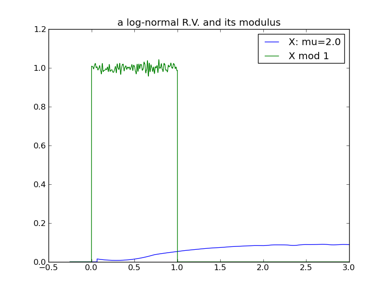
A third example, using a log-normal distribution. The variance of the log-normal increases as a function of both \( \mu \) and \( \sigma \). In this example \( \mu \) is increased systematically, holding \( \sigma \) constant at 1:
 |
 |
 |
 |
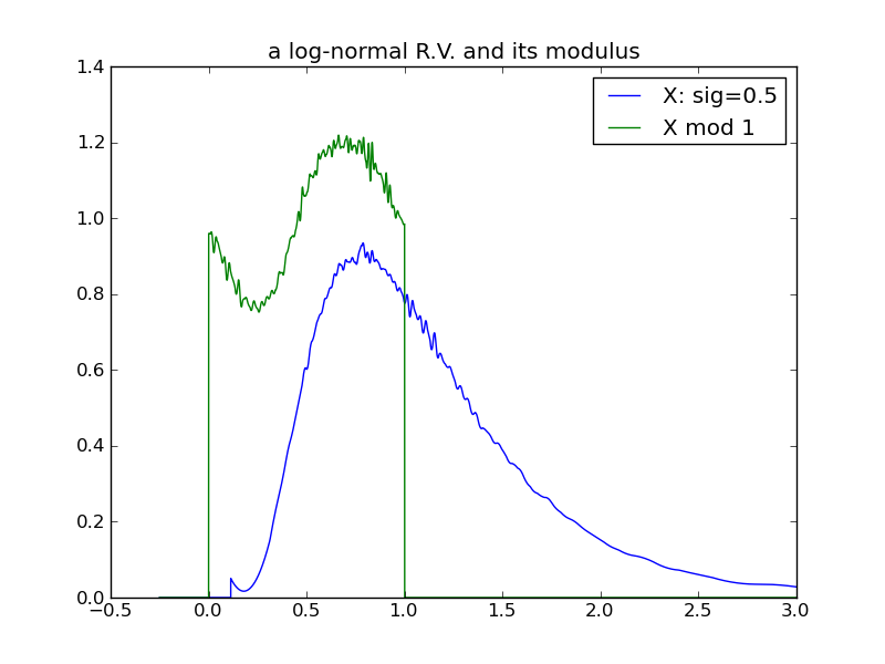
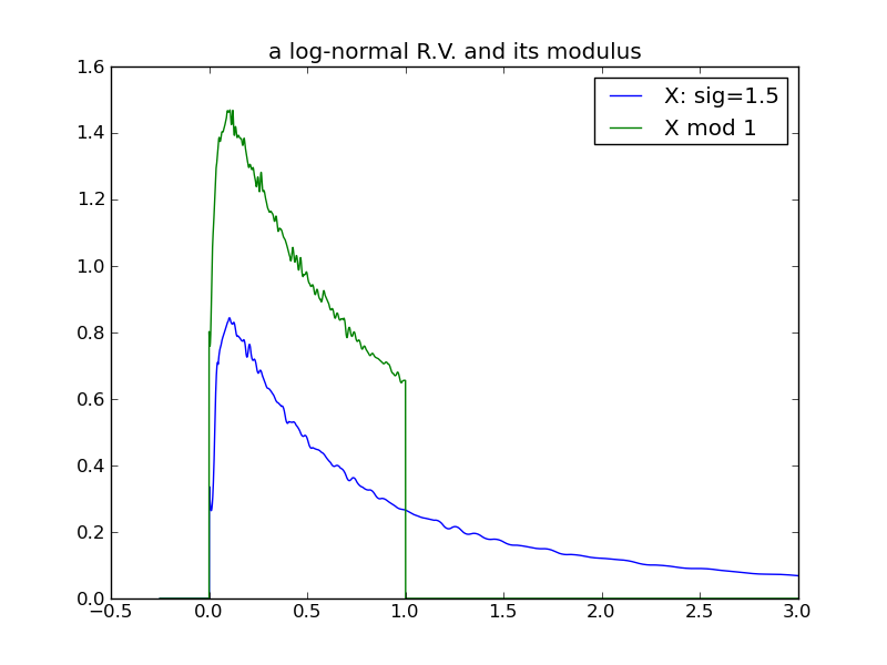
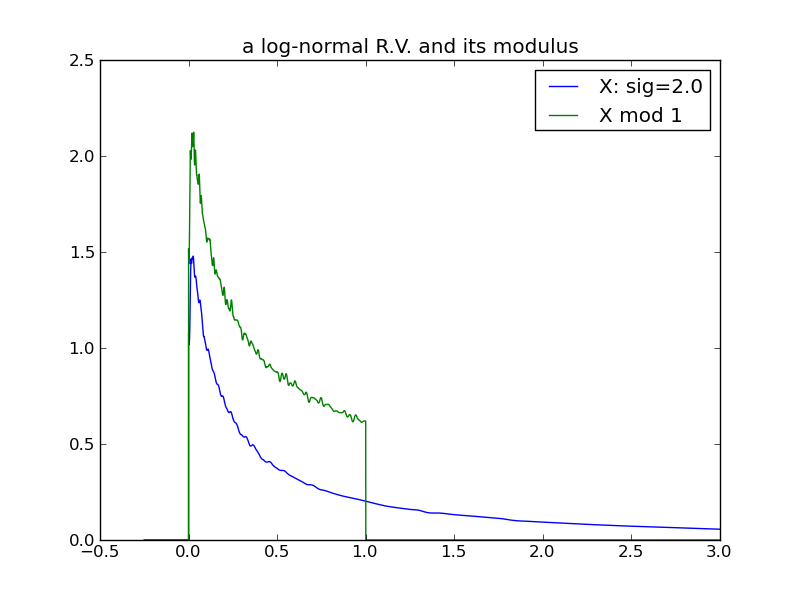
For a final examination of variance, I will again use log-normals and this time vary \( \sigma \), while holding \( \mu \) constant at 0. Here we see that the effect of increasing the log-normal variance via \( \sigma \) does not follow the pattern in previous examples – the distribution does not ‘spread’ and its modulus does not evolve toward a uniform distribution!
 |
|
 |
 |
Modulus and Mean
The following table of plots demonstrates the decreasing effect that a distribution’s location (mean) has, as its spread increases and its modulus approaches uniformity. In fact, we see that any distribution in the ‘uniform modulus’ parameter region is indistinguishable from any other, with respect to its modulus – all changes to mean or variance within this region have no affect on the distribution’s modulus!
 |
 |
 |
 |
 |
 |
 |
 |
 |
Conclusions
Generally, as the spread of a distribution increases, its modulus tends toward a uniform distribution on the modulus interval. Although it was tempting to state this in terms of increasing variance, we see from the 2nd log-normal experiment that variance can increase without increasing ‘spread’ in a way that causes the trend toward uniform modulus. Currently, I’m not sure what the true invariant is, that properly distinguishes the 2nd log-normal scenario from the others.
For any distribution that does reside in the ‘uniform-modulus’ parameter space, we see that neither changes to location nor spread (nor even category of distribution) can be distinguished by the distribution modulus.
Tools
I used the following software widgets:
- rv_modulus_study – the jig for Monte Carlo sampling of underlying distributions and their corresponding modulus
- dplot – a simple cli wrapper around
matplotlib.pyplotfunctionality - Capricious – a library for random sampling of various distribution types
- Capricious::SplineDistribution – a ruby class for estimating PDF and CDF of a distribution from sampled data, using cubic Hermite splines (note, at the time of this writing, I’m using an experimental variation on my personal repo fork, at the link)