 |
Home | Libraries | People | FAQ | More |
#include <boost/math/special_functions/beta.hpp>
namespace boost{ namespace math{

template <class T1, class T2, class T3>
calculated-result-type ibeta(T1 a, T2 b, T3 x);

template <class T1, class T2, class T3, class Policy>
calculated-result-type ibeta(T1 a, T2 b, T3 x, const Policy&);

template <class T1, class T2, class T3>
calculated-result-type ibetac(T1 a, T2 b, T3 x);

template <class T1, class T2, class T3, class Policy>
calculated-result-type ibetac(T1 a, T2 b, T3 x, const Policy&);

template <class T1, class T2, class T3>
calculated-result-type beta(T1 a, T2 b, T3 x);

template <class T1, class T2, class T3, class Policy>
calculated-result-type beta(T1 a, T2 b, T3 x, const Policy&);

template <class T1, class T2, class T3>
calculated-result-type betac(T1 a, T2 b, T3 x);

template <class T1, class T2, class T3, class Policy>
calculated-result-type betac(T1 a, T2 b, T3 x, const Policy&);

}} // namespaces
There are four incomplete beta functions : two are normalised versions (also known as regularized beta functions) that return values in the range [0, 1], and two are non-normalised and return values in the range [0, beta(a, b)]. Users interested in statistical applications should use the normalised (or regularized ) versions (ibeta and ibetac).
All of these functions require 0 <= x <= 1.
The normalized functions ibeta and ibetac require a,b >= 0, and in addition that not both a and b are zero.
The functions beta and betac require a,b > 0.
The return type of these functions is computed using the result type calculation rules when T1, T2 and T3 are different types.
The final Policy argument is optional and can be used to control the behaviour of the function: how it handles errors, what level of precision to use etc. Refer to the policy documentation for more details.
template <class T1, class T2, class T3>
calculated-result-type ibeta(T1 a, T2 b, T3 x);

template <class T1, class T2, class T3, class Policy>
calculated-result-type ibeta(T1 a, T2 b, T3 x, const Policy&);
Returns the normalised incomplete beta function of a, b and x:


template <class T1, class T2, class T3>
calculated-result-type ibetac(T1 a, T2 b, T3 x);

template <class T1, class T2, class T3, class Policy>
calculated-result-type ibetac(T1 a, T2 b, T3 x, const Policy&);
Returns the normalised complement of the incomplete beta function of a, b and x:

template <class T1, class T2, class T3>
calculated-result-type beta(T1 a, T2 b, T3 x);

template <class T1, class T2, class T3, class Policy>
calculated-result-type beta(T1 a, T2 b, T3 x, const Policy&);
Returns the full (non-normalised) incomplete beta function of a, b and x:

template <class T1, class T2, class T3>
calculated-result-type betac(T1 a, T2 b, T3 x);

template <class T1, class T2, class T3, class Policy>
calculated-result-type betac(T1 a, T2 b, T3 x, const Policy&);
Returns the full (non-normalised) complement of the incomplete beta function of a, b and x:

The following tables give peak and mean relative errors in over various domains of a, b and x, along with comparisons to the GSL-1.9 and Cephes libraries. Note that only results for the widest floating-point type on the system are given as narrower types have effectively zero error.
Note that the results for 80 and 128-bit long doubles are noticeably higher than for doubles: this is because the wider exponent range of these types allow more extreme test cases to be tested. For example expected results that are zero at double precision, may be finite but exceptionally small with the wider exponent range of the long double types.
Table 3.8. Errors In the Function ibeta(a,b,x)
|
Significand Size |
Platform and Compiler |
0 < a,b < 10 and 0 < x < 1 |
0 < a,b < 100 and 0 < x < 1 |
1x10⁻⁵ < a,b < 1x10⁵ and 0 < x < 1 |
|---|---|---|---|---|
|
53 |
Win32, Visual C++ 8 |
Peak=42.3 Mean=2.9 (GSL Peak=682 Mean=32.5) (Cephes Peak=42.7 Mean=7.0) |
Peak=108 Mean=16.6 (GSL Peak=690 Mean=151) (Cephes Peak=1545 Mean=218) |
Peak=4x10³ Mean=203 (GSL Peak~3x10⁵ Mean~2x10⁴ ) (Cephes Peak~5x10⁵ Mean~2x10⁴ ) |
|
64 |
Redhat Linux IA32, gcc-3.4.4 |
Peak=21.9 Mean=3.1 |
Peak=270.7 Mean=26.8 |
Peak~5x10⁴ Mean=3x10³ |
|
64 |
Redhat Linux IA64, gcc-3.4.4 |
Peak=15.4 Mean=3.0 |
Peak=112.9 Mean=14.3 |
Peak~5x10⁴ Mean=3x10³ |
|
113 |
HPUX IA64, aCC A.06.06 |
Peak=20.9 Mean=2.6 |
Peak=88.1 Mean=14.3 |
Peak~2x10⁴ Mean=1x10³ |
Table 3.9. Errors In the Function ibetac(a,b,x)
|
Significand Size |
Platform and Compiler |
0 < a,b < 10 and 0 < x < 1 |
0 < a,b < 100 and 0 < x < 1 |
1x10⁻⁵ < a,b < 1x10⁵ and 0 < x < 1 |
|---|---|---|---|---|
|
53 |
Win32, Visual C++ 8 |
Peak=13.9 Mean=2.0 |
Peak=56.2 Mean=14 |
Peak=3x10³ Mean=159 |
|
64 |
Redhat Linux IA32, gcc-3.4.4 |
Peak=21.1 Mean=3.6 |
Peak=221.7 Mean=25.8 |
Peak~9x10⁴ Mean=3x10³ |
|
64 |
Redhat Linux IA64, gcc-3.4.4 |
Peak=10.6 Mean=2.2 |
Peak=73.9 Mean=11.9 |
Peak~9x10⁴ Mean=3x10³ |
|
113 |
HPUX IA64, aCC A.06.06 |
Peak=9.9 Mean=2.6 |
Peak=117.7 Mean=15.1 |
Peak~3x10⁴ Mean=1x10³ |
Table 3.10. Errors In the Function beta(a, b, x)
|
Significand Size |
Platform and Compiler |
0 < a,b < 10 and 0 < x < 1 |
0 < a,b < 100 and 0 < x < 1 |
1x10⁻⁵ < a,b < 1x10⁵ and 0 < x < 1 |
|---|---|---|---|---|
|
53 |
Win32, Visual C++ 8 |
Peak=39 Mean=2.9 |
Peak=91 Mean=12.7 |
Peak=635 Mean=25 |
|
64 |
Redhat Linux IA32, gcc-3.4.4 |
Peak=26 Mean=3.6 |
Peak=180.7 Mean=30.1 |
Peak~7x10⁴ Mean=3x10³ |
|
64 |
Redhat Linux IA64, gcc-3.4.4 |
Peak=13 Mean=2.4 |
Peak=67.1 Mean=13.4 |
Peak~7x10⁴ Mean=3x10³ |
|
113 |
HPUX IA64, aCC A.06.06 |
Peak=27.3 Mean=3.6 |
Peak=49.8 Mean=9.1 |
Peak~6x10⁴ Mean=3x10³ |
Table 3.11. Errors In the Function betac(a,b,x)
|
Significand Size |
Platform and Compiler |
0 < a,b < 10 and 0 < x < 1 |
0 < a,b < 100 and 0 < x < 1 |
1x10⁻⁵ < a,b < 1x10⁵ and 0 < x < 1 |
|---|---|---|---|---|
|
53 |
Win32, Visual C++ 8 |
Peak=12.0 Mean=2.4 |
Peak=91 Mean=15 |
Peak=4x10³ Mean=113 |
|
64 |
Redhat Linux IA32, gcc-3.4.4 |
Peak=19.8 Mean=3.8 |
Peak=295.1 Mean=33.9 |
Peak~1x10⁵ Mean=5x10³ |
|
64 |
Redhat Linux IA64, gcc-3.4.4 |
Peak=11.2 Mean=2.4 |
Peak=63.5 Mean=13.6 |
Peak~1x10⁵ Mean=5x10³ |
|
113 |
HPUX IA64, aCC A.06.06 |
Peak=15.6 Mean=3.5 |
Peak=39.8 Mean=8.9 |
Peak~9x10⁴ Mean=5x10³ |
There are two sets of tests: spot tests compare values taken from Mathworld's online function evaluator with this implementation: they provide a basic "sanity check" for the implementation, with one spot-test in each implementation-domain (see implementation notes below).
Accuracy tests use data generated at very high precision (with NTL RR class set at 1000-bit precision), using the "textbook" continued fraction representation (refer to the first continued fraction in the implementation discussion below). Note that this continued fraction is not used in the implementation, and therefore we have test data that is fully independent of the code.
This implementation is closely based upon "Algorithm 708; Significant digit computation of the incomplete beta function ratios", DiDonato and Morris, ACM, 1992.
All four of these functions share a common implementation: this is passed both x and y, and can return either p or q where these are related by:

so at any point we can swap a for b, x for y and p for q if this results in a more favourable position. Generally such swaps are performed so that we always compute a value less than 0.9: when required this can then be subtracted from 1 without undue cancellation error.
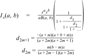
The following continued fraction representation is found in many textbooks but is not used in this implementation - it's both slower and less accurate than the alternatives - however it is used to generate test data:

The following continued fraction is due to Didonato and Morris, and is used in this implementation when a and b are both greater than 1:

For smallish b and x then a series representation can be used:

When b << a then the transition from 0 to 1 occurs very close to x = 1 and some care has to be taken over the method of computation, in that case the following series representation is used:

Where Q(a,x) is an incomplete gamma function. Note that this method relies on keeping a table of all the pn previously computed, which does limit the precision of the method, depending upon the size of the table used.
When a and b are both small integers, then we can relate the incomplete beta to the binomial distribution and use the following finite sum:

Finally we can sidestep difficult areas, or move to an area with a more efficient means of computation, by using the duplication formulae:


The domains of a, b and x for which the various methods are used are identical to those described in the Didonato and Morris TOMS 708 paper.