 |
Home | Libraries | People | FAQ | More |
#include <boost/math/distributions/triangular.hpp>
namespace boost{ namespace math{
 template <class RealType = double,
           class Policy   = policies::policy<> >
 class triangular_distribution;

 typedef triangular_distribution<> triangular;

 template <class RealType, class Policy>
 class triangular_distribution
 {
 public:
    typedef RealType value_type;
    typedef Policy   policy_type;

    triangular_distribution(RealType lower = -1, RealType mode = 0) RealType upper = 1); // Constructor.
       : m_lower(lower), m_mode(mode), m_upper(upper) // Default is -1, 0, +1 triangular distribution.
    // Accessor functions.
    RealType lower()const;
    RealType mode()const;
    RealType upper()const;
 }; // class triangular_distribution

}} // namespaces
The triangular distribution is a continuous probability distribution with a lower limit a, mode c, and upper limit b.
The triangular distribution is often used where the distribution is only vaguely known, but, like the uniform distribution, upper and limits are 'known', but a 'best guess', the mode or center point, is also added. It has been recommended as a proxy for the beta distribution. The distribution is used in business decision making and project planning.
The triangular distribution is a distribution with the probability density function:
f(x) =
Parameter a (lower) can be any finite value. Parameter b (upper) can be any finite value > a (lower). Parameter c (mode) a <= c <= b. This is the most probable value.
The random variate x must also be finite, and is supported lower <= x <= upper.
The triangular distribution may be appropriate when an assumption of a normal distribution is unjustified because uncertainty is caused by rounding and quantization from analog to digital conversion. Upper and lower limits are known, and the most probable value lies midway.
The distribution simplifies when the 'best guess' is either the lower or upper limit - a 90 degree angle triangle. The default chosen is the 001 triangular distribution which expresses an estimate that the lowest value is the most likely; for example, you believe that the next-day quoted delivery date is most likely (knowing that a quicker delivery is impossible - the postman only comes once a day), and that longer delays are decreasingly likely, and delivery is assumed to never take more than your upper limit.
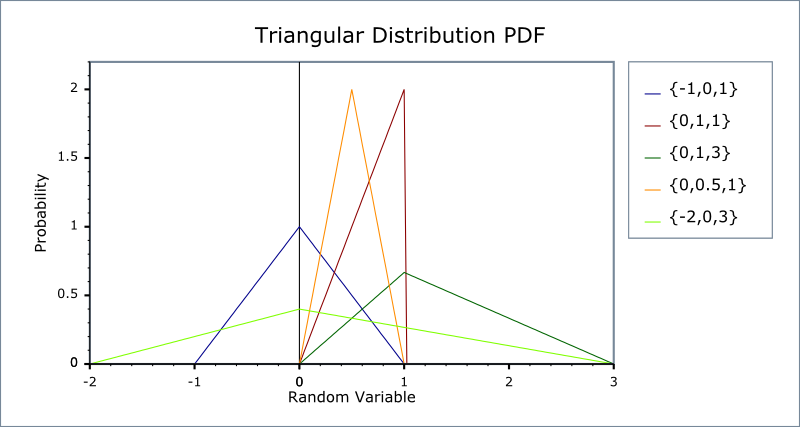
The following graph illustrates how the probability density function PDF varies with the various parameters:

and cumulative distribution function

triangular_distribution(RealType lower = 0, RealType mode = 0 RealType upper = 1);
Constructs a triangular distribution with lower lower (a) and upper upper (b).
Requires that the lower, mode and upper parameters are all finite, otherwise calls domain_error.
RealType lower()const;
Returns the lower parameter of this distribution (default -1).
RealType mode()const;
Returns the mode parameter of this distribution (default 0).
RealType upper()const;
Returns the upper parameter of this distribution (default+1).
All the usual non-member accessor functions that are generic to all distributions are supported: Cumulative Distribution Function, Probability Density Function, Quantile, Hazard Function, Cumulative Hazard Function, mean, median, mode, variance, standard deviation, skewness, kurtosis, kurtosis_excess, range and support.
The domain of the random variable is \lowerto \upper, and the supported range is lower <= x <= upper.
The triangular distribution is implemented with simple arithmetic operators and so should have errors within an epsilon or two, except quantiles with arguments nearing the extremes of zero and unity.
In the following table, a is the lower parameter of the distribution, c is the mode parameter, b is the upper parameter, x is the random variate, p is the probability and q = 1-p.
|
Function |
Implementation Notes |
|---|---|
|
|
Using the relation: pdf = 0 for x < mode, 2(x-a)/(b-a)(c-a) else 2*(b-x)/((b-a)(b-c)) |
|
cdf |
Using the relation: cdf = 0 for x < mode (x-a)2/((b-a)(c-a)) else 1 - (b-x)2/((b-a)(b-c)) |
|
cdf complement |
Using the relation: q = 1 - p |
|
quantile |
let p0 = (c-a)/(b-a) the point of inflection on the cdf, then given probability p and q = 1-p: x = sqrt((b-a)(c-a)p) + a ; for p < p0 x = c ; for p == p0 x = b - sqrt((b-a)(b-c)q) ; for p > p0 (See /boost/math/distributions/triangular.hpp for details.) |
|
quantile from the complement |
As quantile (See /boost/math/distributions/triangular.hpp for details.) |
|
mean |
(a + b + 3) / 3 |
|
variance |
(a2+b2+c2 - ab - ac - bc)/18 |
|
mode |
c |
|
skewness |
(See /boost/math/distributions/triangular.hpp for details). |
|
kurtosis |
12/5 |
|
kurtosis excess |
-3/5 |
Some 'known good' test values were obtained from Statlet: Calculate and plot probability distributions