 |
Home | Libraries | People | FAQ | More |
#include <boost/math/distributions/logistic.hpp>
namespace boost{ namespace math{

template <class RealType = double,
          class Policy   = policies::policy<> >
class logistic_distribution;

template <class RealType, class Policy>
class logistic_distribution
{
public:
   typedef RealType value_type;
   typedef Policy   policy_type;
   // Construct:
   logistic_distribution(RealType location = 0, RealType scale = 1);
   // Accessors:
   RealType location()const; // location.
   RealType scale()const; // scale.

};

typedef logistic_distribution<> logistic;

}} // namespaces
The logistic distribution is a continous probability distribution. It has two parameters - location and scale. The cumulative distribution function of the logistic distribution appears in logistic regression and feedforward neural networks. Among other applications, United State Chess Federation and FIDE use it to calculate chess ratings.
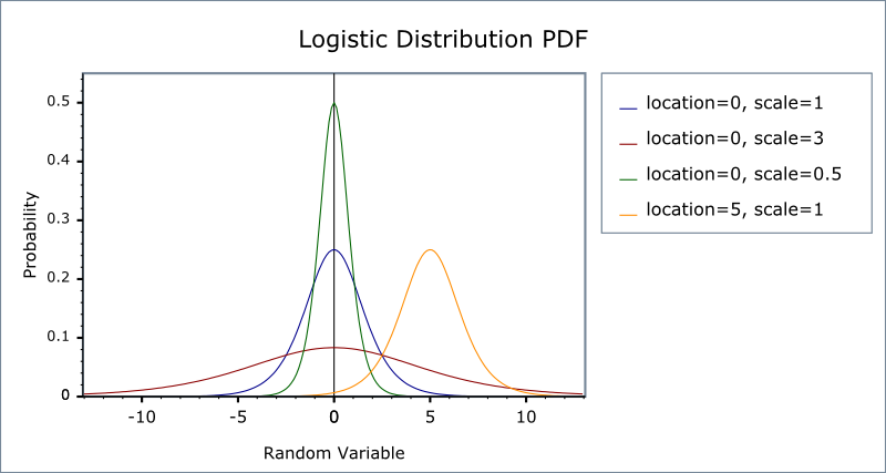
The following graph shows how the distribution changes as the parameters change:

logistic_distribution(RealType u = 0, RealType s = 1);
Constructs a logistic distribution with location u and scale s.
Requires scale >
0, otherwise a domain_error
is raised.
RealType location()const;
Returns the location of this distribution.
RealType scale()const;
Returns the scale of this distribution.
All the usual non-member accessor functions that are generic to all distributions are supported: Cumulative Distribution Function, Probability Density Function, Quantile, Hazard Function, Cumulative Hazard Function, mean, median, mode, variance, standard deviation, skewness, kurtosis, kurtosis_excess, range and support.
The domain of the random variable is [-[max_value], +[min_value]]. However, the pdf and cdf support inputs of +∞ and -∞ as special cases if RealType permits.
At p=1 and p=0, the quantile
function returns the result of +overflow_error
and -overflow_error,
while the complement quantile function returns the result of -overflow_error
and +overflow_error
respectively.
The logistic distribution is implemented in terms of the std::exp and the std::log
functions, so its accuracy is related to the accurate implementations of
those functions on a given platform. When calculating the quantile with
a non-zero position parameter catastrophic cancellation
errors can occur: in such cases, only a low absolute error
can be guarenteed.
|
Function |
Implementation Notes |
|---|---|
|
|
Using the relation: pdf = e-(x-u)/s / (s*(1+e-(x-u)/s)2) |
|
cdf |
Using the relation: p = 1/(1+e-(x-u)/s) |
|
cdf complement |
Using the relation: q = 1/(1+e(x-u)/s) |
|
quantile |
Using the relation: x = u - s*log(1/p-1) |
|
quantile from the complement |
Using the relation: x = u + s*log(p/1-p) |
|
mean |
u |
|
mode |
The same as the mean. |
|
skewness |
0 |
|
kurtosis excess |
6/5 |
|
variance |
(π*s)2 / 3 |