Very Fast Reservoir Sampling
In this post I will demonstrate how to do reservoir sampling orders of magnitude faster than the traditional “naive” reservoir sampling algorithm, using a fast high-fidelity approximation to the reservoir sampling-gap distribution.
The code I used to collect the data for this post can be viewed here. I generated the plots using the quantifind WISP project.
Update (April 4, 2016): my colleague RJ Nowling ran across a paper by J.S. Vitter that shows Vitter developed the trick of accelerating sampling with a sampling-gap distribution in 1987 – I re-invented Vitter’s wheel 30 years after the fact! I’m surprised it never caught on, as it is not much harder to implement than the naive version.
In a previous post, I showed that random Bernoulli and Poisson sampling could be made much faster by modeling the sampling gap distribution for the corresponding sampling distributions. More recently, I also began exploring whether reservoir sampling might also be optimized using the gap sampling technique, by deriving the reservoir sampling gap distribution. For a sampling reservoir of size (R), starting at data element (j), the probability distribution of the sampling gap is:

Modeling a sampling gap distribution is a powerful tool for optimizing a sampling algorithm, but it presupposes that you can actually draw values from that distribution substantially faster than just applying a random process to drawing each data element. I was unable to come up with a “direct” algorithm for drawing samples from P(k) above (I suspect none exists), however I also know the CDF F(k), so it is possible to apply inversion sampling, which runs in logarithmic time w.r.t the desired accuracy. Although its logarithmic cost effectively guarantees that it will be a net efficiency win for sufficiently large (j), it still involves a substantial number of computations to yield its samples, and it seems unlikely to be competitive with straight “naive” reservoir sampling over many real-world data sizes, where (j) may never grow very large.
Well, if exact computations are too expensive, we can always look for a fast approximation. Consider the original “first principles” formula for the sampling gap P(k):

As the figure above alludes to, if (j) is relatively large compared to (k), then values (j+1),(j+2)…(j+k) are all going to be effectively “close” to (j), and so we can replace them all with (j) as an approximation. Note that the resulting approximation is just the PMF of the geometric distribution, with probability of success p=(R/j), and we already saw how to efficiently draw values from a geometric distribution from our experience with Bernoulli sampling.
Do we have any reason to hope that this approximation will be useful? For reasons that are similar to those for Bernoulli gap sampling, it will only be efficient to employ gap sampling when the probability (R/j) becomes small enough. From our experiences with Bernoulli sampling that is at least j>=2R. So, we have some assurance that (j) itself will be never be very small. What about (k)? Note that a geometric distribution “favors” smaller values of (k) – that is, small values of (k) have the highest probabilities. In fact, the smaller that (j) is, the larger the probability (R/j) is, and so the more likely that (k) values that are small relative to (j) will be the frequent ones. It is also promising that the true distribution for P(k) also favors smaller values of (k) (in fact it favors them even a bit more strongly than the approximation).
Although it is encouraging, it is also clear that my argument above is limited to heuristic hand-waving. What does this approximation really look like, compared to the true distribution? Fortunately, it is easy to plot both distributions numerically, since we now know the formulas for both:
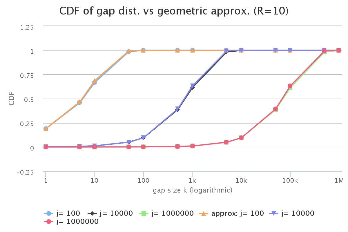
The plot above shows that, in fact, the geometric approximation is a surprisingly good approximation to the true distribution! Furthermore, the approximation remains good as both (j) and (k) grow larger.
Our numeric eye-balling looks quite promising. Is there an effective way to measure how good this approximation is? One useful measure is the Kolmogorov-Smirnov D statistic, which is just the maximum absolute error between two cumulative distributions. Here is a plot of the D statistic for reservoir size R=10, as (j) varies across several magnitudes:
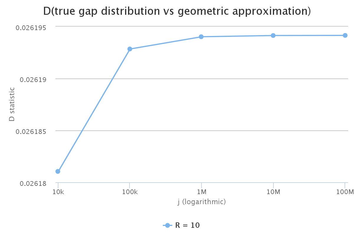
This plot is also good news: we can see that deviation, as measured by D, remains bounded at a small value (less than 0.0262). As this is for the specific value R=10, we also want to know how things change as reservoir size changes:
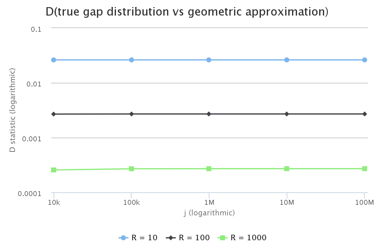
The news is still good! As reservoir size grows, the approximation only gets better: the D values get smaller as R increases, and remain asymptotically bounded as (j) increases.
Now we have some numeric assurance that the geometric approximation is a good one, and stays good as reservoir size grows and sampling runs get longer. However, we should also verify that an actual implementation of the approximation works as expected.
Here is pseudocode for an implementation of reservoir sampling using the fast geometric approximation:
// data is array to sample from
// R is the reservoir size
function reservoirFast(data: Array, R: Int) {
  n = data.length
  // Initialize reservoir with first R elements of data:
  res = data[0 until R]
  // Until this threshold, use traditional sampling.  This value may
  // depend on performance characteristics of random number generation and/or
  // numeric libraries:
  t = 4 * R
  j = 1 + R
  while (j < n  &&  j <= t) {
    k = randomInt(j) // random integer >= 0 and < j
    if (k < R) res[k] = data[j]
    j = j + 1
  }
  // Once gaps become significant, it pays to do gap sampling
  while (j < n) {
    // draw gap size (g) from geometric distribution with probability p = R/j
    p = R / j
    u = randomFloat() // random float > 0 and <= 1
    g = floor(log(u) / log(1-p))
    j = j + g
    if (j < n) {
      k = randomInt(R)
      res[k] = data[j]
    }
    j = j + 1
  }
  // return the reservoir
  return res
}
Following is a plot that shows two-sample D statistics, comparing the distribution in sample gaps between runs of the exact “naive” reservoir sampling with the fast geometric approximation:
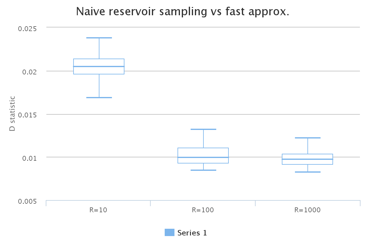
As expected, the measured difference in sampling characteristics between naive and fast approximation are small, confirming the numeric predictions.
Since the point of this exercise was to achieve faster random sampling, it remains to measure what kind of speed improvements the fast approximation provides. As a point of reference, here is a plot of run times for reservoir sampling over 10^8 integers:
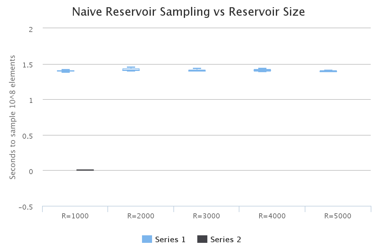
As expected, sample time remains constant at around 1.5 seconds, regardless of reservoir size, since the naive algorithm always samples from its RNG per each sample.
Compare this to the corresponding plot for the fast geometric approximation:
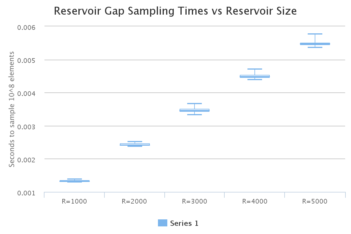
Firstly, we see that the sampling times are much faster, as originally anticipated in my previous post – in the neighborhood of 3 orders of magnitude faster. Secondly, we see that the sampling times do increase as a linear function of reservoir size. Based on our experience with Bernoulli gap sampling, this is expected; the sampling probabilities are given by (R/j), and therefore the amount of sampling is proportional to R.
Another property anticipated in my previous post was that the efficiency of gap sampling should continue to increase as the amount of data sampled grows; the sampling probability being (R/j), the probability of sampling decreases as j gets larger, and so the corresponding gap sizes grow. The following plot verifies this property, holding reservoir size R constant, and increasing the data size:
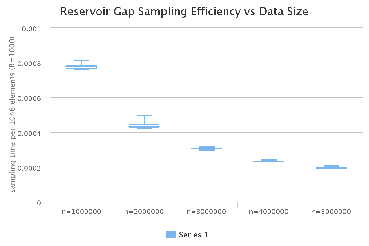
The sampling time (per million elements) decreases as the sample size grows, as predicted by the formula.
In conclusion, I have demonstrated that a geometric distribution can be used as a high quality approximation to the true sampling gap distribution for reservoir sampling, which allows reservoir sampling to be performed much faster than the naive algorithm while still retaining sampling quality.