The Reservoir Sampling Gap Distribution
In a previous post, I showed that random Bernoulli and Poisson sampling could be made much faster by modeling the sampling gap distribution - that is, directly drawing random samples from the distribution of how many elements would be skipped over between actual samples taken.
Another popular sampling algorithm is Reservoir Sampling. Its sampling logic is a bit more complicated than Bernoulli or Poisson sampling, in the sense that the probability of sampling any given (jth) element changes. For a sampling reservoir of size R, and all j>R, the probability of choosing element (j) is R/j. You can see that the potential payoff for gap-sampling is big, particularly as data size becomes large; as (j) approaches infinity, the probability R/j goes to zero, and the corresponding gaps between samples grow without bound.
Modeling a sampling gap distribution is a powerful tool for optimizing a sampling algorithm, but it requires that (1) you actually know the sampling distribution, and (2) that you can effectively draw values from that distribution faster than just applying a random process to drawing each data element.
With that goal in mind, I derived the probability mass function (pmf) and cumulative distribution function (cdf) for the sampling gap distribution of reservoir sampling. In this post I will show the derivations.
The Sampling Gap Distribution
In the interest of making it easy to get at the actual answers, here are the pmf and cdf for the Reservoir Sampling Gap Distribution. For a sampling reservoir of size (R), starting at data element (j), the probability distribution of the sampling gap is:

Conventions
In the derivations that follow, I will keep to some conventions:
- R = the sampling reservoir size. R > 0.
- j = the index of a data element being considered for sampling. j > R.
- k = the size of a gap between samples. k >= 0.
P(k) is the probability that the gap between one sample and the next is of size k. The support for P(k) is over all k>=0. I will generally assume that j>R, as the first R samples are always loaded into the reservoir and the actual random sampling logic starts at j=R+1. The constraint j>R will also be relevant to many binomial coefficient expressions, where it ensures the coefficient is well defined.
Deriving the Probability Mass Function, P(k)
Suppose we just chose (randomly) to sample data element (j-1). Now we are interested in the probability distribution of the next sampling gap. That is, the probability P(k) that we will not sample the next (k) elements {j,j+1,…j+k-1}, and sample element (j+k):

By arranging the product terms in descending order as above, you can see that they can be written as factorial quotients:
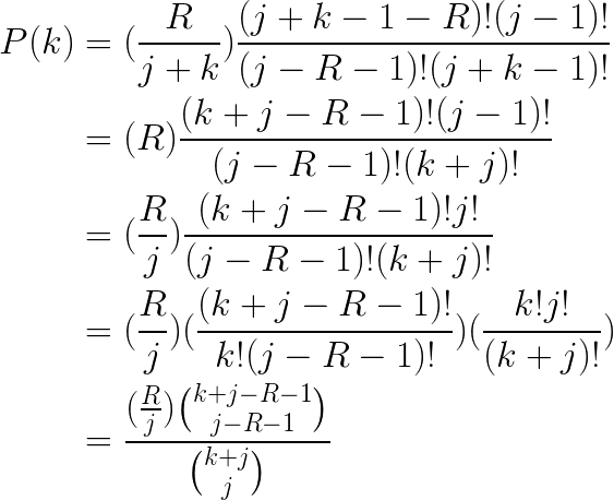
Now we apply Lemma A. The 2nd case (a<=b) of the Lemma applies, since (j-1-R)<=j, so we have:
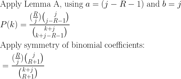
And so we have now derived a compact, closed-form expression for P(k).
Deriving the Cumulative Distribution Function, F(k)
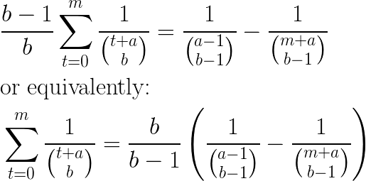
Now that we have a derivation for the pmf P(k), we can tackle a derivation for the cdf. First I will make note of this useful identity that I scraped off of Wikipedia (I substituted (x) => (a) and (k) => (b)):
The cumulative distribution function for the sampling gap, F(k), is of course just the sum over P(t), for (t) from 0 up to (k):
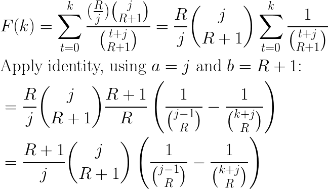
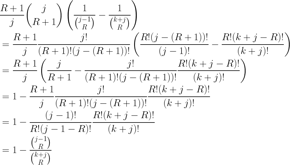
This is a closed-form solution, but we can apply a bit more simplification:
Conclusions
We have derived closed-form expressions for the pmf and cdf of the Reservoir Sampling gap distribution:

In order to apply these results to a practical gap-sampling implementation of Reservoir Sampling, we would next need a way to efficiently sample from P(k), to obtain gap sizes to skip over. How to accomplish this is an open question, but knowing a formula for P(k) and F(k) is a start.
Acknowledgements
Many thanks to RJ Nowling and Will Benton for proof reading and moral support! Any remaining errors are my own fault.
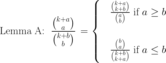
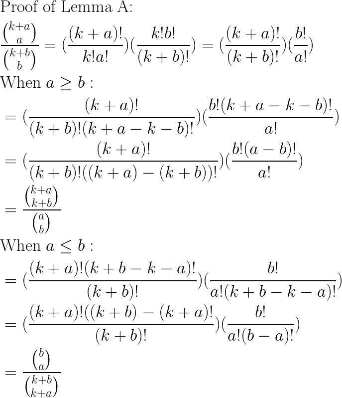
Lemma A, And Its Proof
